Configure Time Scope Block
When you use the Time Scope block, you can configure many settings and tools from the scope window. The following sections show how to use the Time Scope interface and the available tools.
Signal Display
These figures highlight the important aspects of the Time Scope window in Simulink®.
Scope Tab
Measurements Tab
Title, Y-Axis Label — You can customize the title and the y-axis label from Settings.
Toolstrip
Scope tab — Customize and share the time scope. For example, showing and hiding the legend.
Measurements tab — Turn on and control different measurement tools.
Use the pin button
 to pin the toolstrip or the arrow button
 to hide the toolstrip.
Time Indicators
Min Time-Axis Limit — Time Scope sets the minimum time-axis (x-axis) limit using the value of the Time display offset parameter. To change the Time display offset value, click Settings (
 ) in the Scope tab of the
toolstrip. Under Time, set Time display
offset.
) in the Scope tab of the
toolstrip. Under Time, set Time display
offset.Max Time-Axis Limit — Time Scope sets the maximum time-axis (x-axis) limit by adding the values of the Time display offset and Time span parameters. If you specify a vector of values in Time display offset, the scope sets the maximum time-axis limit by adding the largest value in the vector to the value of the Time span parameter.
For example, if you set Time span to
25seconds, the scope displays 25 seconds of simulation data at a time. If you also set Time display offset to5seconds, the scope displays values on the time axis from5to30seconds.The values on the time axis of the Time Scope display remain the same throughout simulation.
Time Units –– Units to describe the time-axis. The Time Scope sets the time units using the value of the Time units parameter under Settings > Time. By default, this parameter is set to
Metric (based on Time
                            Span)
and displays in metric units such as milliseconds, microseconds, minutes, days, etc. You can change it toSecondsto always display the time-axis values in units of seconds. You can change it toNoneto not display any units on the time axis. When you set this parameter toNone, then Time Scope shows only the wordTimeon the time axis.To hide both the word
Timeand the values on the time axis, set the T-axis and tick labels toNone. To hide both the wordTimeand the values on the time axis in all displays, except the bottom ones in each column of displays, set this parameter toBottom displays only. This behavior differs from the Simulink Scope (Simulink) block, which always shows the values but never shows a label on the x-axis.
Simulation Indicators
Simulation Status — Provide model simulation status in the status bar in the scope window. The status can be:
Ready–– Occurs after you open the scope and before your first run a simulation.Running–– Occurs during the simulation.
Time Offset — The
Offsetvalue on the status bar helps you determine the simulation times for which the scope is displaying data. The value is always in the range0≤Offset≤ Simulation Time. If the time offset is 0, the Scope does not display theOffsetstatus field. Add the time offset to the fixed time span values on the time-axis to get the overall simulation time.For example, if you set the Time span to
20seconds, and you see anOffsetof0on the scope window. This value indicates that the scope is displaying data for the first0to20seconds of simulation time. If theOffsetchanges to20, the scope displays data for simulation times from20seconds to40seconds. The scope continues to update theOffsetvalue until the simulation is complete.Simulation Time — The amount of time that the Time Scope has spent processing the input. Every time you call the scope, the simulation time increases by the number of rows in the input signal divided by the sample rate, as given by the following formula: . Sample rate is the inverse of the Sample time value that you set under Settings > Time.
The Simulation Time parameter is located on the status bar in the Time Scope window.
Display Multiple Signals
Multi-Signal Input
You can configure the Time Scope to show multiple signals within the same display or in separate displays. By default, the signals appear as different colored lines on the same display. The signals can have different dimensions, sample rates, and data types. Each signal can be real or complex valued. You can set the number of input ports on the Time Scope in the following ways:
Set Number of input ports under Settings > General in the Scope tab of the toolstrip.
Add signal lines to the scope directly.
An input signal may contain multiple channels, depending on its dimensions. Multiple channels of data always appear as different colored lines in the same display.
Multiple Signal Names and Colors. By default, if the input signal has multiple channels, the scope uses an index
number to identify each channel of that signal. For example, a 2-channel signal
will have the following default names in the channel legend: Channel
1 and Channel 2. The scope displays all the
channels of the signal on a single display. To show the signal legend, select
Show legend under Settings >
Display in the Scope tab of the
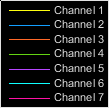
toolstrip. If there are a total of seven input channels, the following legend
appears in the display.
By default, the scope has a black axes background and it selects line colors for each channel in a manner similar to the Simulink Scope (Simulink) block. When the scope axes background is black, it assigns each channel of each input signal a line color in the order shown in this figure.
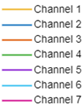
If there are more than seven channels, then the scope repeats this order to assign line colors to the remaining channels. To choose line colors for each channel, change the axes background color to any color except black. For example, to change the axes background color to white, click the Axes background drop-down arrow and select white from the color palette. You can find Axes background under Settings > Axes Style in the Scope tab of the toolstrip. Run the simulation again. The following legend appears in the display. This figure shows the color order when the background is not black.
Multiple Displays
You can display multiple signals on different displays in the scope window. For example, if there are two inputs to the scope, you can display the signals in two separate displays. To customize the display layout:
Set Display grid under Settings > General in the Scope tab of the toolstrip to a two-element numeric vector with each element greater than 0 and less than or equal to 16. For example, setting Display grid to [
21] changes the layout to a 2-by-1 grid.Click the Display Grid in the Scope tab of the toolstrip and select a layout using the grid picker. The grid picker allows you to select up to a 5-by-5 grid.
If the number of displays is equal to the number of ports, signals from each port appear on separate displays. If the number of displays is less than the number of ports, signals from additional ports appear on the last display. For layouts with multiple columns and rows, ports are mapped down then across. If the number of displays is greater than the number of ports, the scope creates empty tiles.
When there is more than one display, the scope enables the Active Display parameter under Settings. Using this parameter, you can select which display to update based on the Line Style, Y-axis, and Display settings.
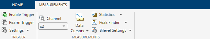
Time Scope Measurements
The Time Scope measurement panels show the signal measurements for a specified channel and these panels appear at the bottom of the scope UI. To open a measurement panel, you must first enable the corresponding measurement in the scope toolstrip.
The Time Scope block supports these measurements:
Triggers — Set triggers to sync repeating signals and pause the display when events occur.
Cursor Measurements — Measure signal values using vertical and horizontal cursors.
Signal Statistics — Display the maximum, minimum, peak-to-peak difference, mean, median, and RMS values of a selected signal.
Peak Finder — Find maxima, showing the x-axis values at which they occur.
Bilevel Measurements — Measure transitions, overshoots, undershoots, and cycles.
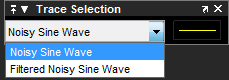
The Time Scope computes measurements for the specified channel. By default, the scope applies the measurements to the first channel. To change the channel, use the Channel Selector in the Measurements tab.
When you input multiple signals to the scope, the scope enables the Channel Selector in the Measurements tab. Select the signal to measure from the drop-down options of the channel selector.
Scope Window Management
Dock multiple scope windows of a Simulink model into a single window called the scope container. The scope container provides a unified view for all the scope displays in the model and enables you to manage and organize multiple scopes in a single window. The settings in the Home tab and the Measurements tab apply only to the active scope, that is, the scope in the container that you are actively interacting with.
Home Tab
The Home tab of the scope container is similar to the Scope tab of the Time Scope block toolstrip.
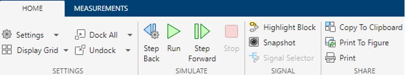
Settings
Click Settings to launch the Style Settings side panel for the currently active scope. In this panel, you can control all the scope related settings, such as general settings, time and axes settings, display settings, style settings, and settings related to logging. For more information on these properties, see Settings in the Time Scope reference page.
Legend
Click Settings > Legend to show the signal legend on the active scope.
Display Grid
Opens a grid picker similar to the scope layout. The layout can have a maximum of 16 rows and 16 columns.
If the number of displays is equal to the number of ports, signals from each port appear on separate displays. If the number of displays is less than the number of ports, signals from additional ports appear in the last display. For layouts with multiple columns and rows, the scope maps ports down then across. If the number of displays is greater than the number of ports, the scope creates empty tiles.
Dock All
Click Dock All to add all the opened scopes in the current model to the scope container. To automatically add newly opened scopes to the existing scope container, select Dock All > Dock New Scopes on Open.
Undock
Click Undock to remove the currently active scope from the container into a separate standalone window. When there are multiple scope windows in the container, click Undock > Undock All to remove all scopes from the container into separate standalone windows.
Measurements Tab
The Measurements tab of the scope container is similar to the Measurements tab of the Time Scope block toolstrip.
Share or Save the Time Scope
If you want to save the time scope for future use or share it with others, use the buttons in the Share section of the Scope tab.
Copy to Clipboard — Copy the display to your clipboard. You can paste the image in another program to save or share it.
Print to Figure –– Print to a MATLAB® figure.
Print — Opens a print dialog box from which you can print out the plot image.
Scale Axes
To scale the plot axes, you can use the mouse to pan around the axes and the scroll button on your mouse to zoom in and out of the plot. Additionally, you can use the buttons that appear when you hover over the plot window.
 — Pan the plot.
 — Zoom in and out of the plot.
 — Autoscale the axes to fit the shown
data.
— Autoscale the axes to fit the shown
data.