Scope
Display signals generated during simulation
Libraries:
Simulink /
Commonly Used Blocks
Simulink /
Sinks
HDL Coder /
Commonly Used Blocks
HDL Coder /
Sinks
Description
The Simulink® Scope block and DSP System Toolbox™ Time Scope block display time domain signals.
The two blocks have identical functionality, but different default settings. The Time Scope is optimized for discrete-time processing. The Scope is optimized for general time-domain simulation. For a side-by-side comparison, see Simulink Scope Block Versus DSP System Toolbox Time Scope Block.
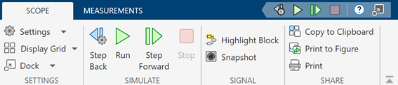
Scope Tab
This image highlights the important aspects of the scope window.
Scope display features:
Simulation control — Run and debug models from a Scope window using Run, Step Forward, and Step Backward toolbar buttons.
Multiple signals — Plot multiple signals on the same display using multiple input ports.
Multiple displays — Display signals on multiple subplots. All the y-axes of the subplots have a common time range on the x-axis. Control the layout of the subplots using the Display Grid parameter in the Scope tab of the toolstrip.
Modify parameters — Modify scope parameter values before and during a simulation.
Axis autoscaling — Autoscale axes during or at the end of a simulation. Margins are drawn at the top and bottom of the axes.
Display data after simulation — The scope saves data during a simulation. If you close a scope when simulation starts and open it after simulation ends, the scope displays simulation results for attached input signals.
Note
If you have a high sample rate or the simulation time is long, you can run into issues with memory or system performance because the scope saves data internally. To limit the amount of data saved by the scope for visualization, use the
Limit data points to lastparameter.Scope window management –– The scope container enables you to dock multiple scopes from a Simulink model into a single window. The container provides a convenient interface from which you can visualize the signals and manage the settings of the scopes.
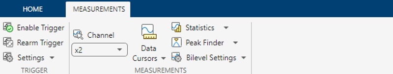
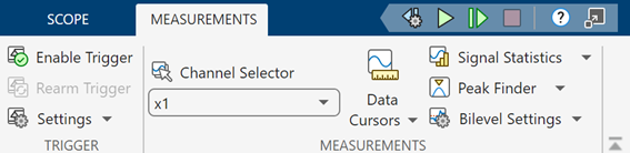
Measurements Tab
This image highlights the important aspects of the measurements window.
The Scope block supports these measurements:
Triggers — Set triggers to sync repeating signals and pause the display when events occur.
Cursor Measurements — Measure signal values using vertical and horizontal cursors.
Signal Statistics — Display the maximum, minimum, peak-to-peak difference, mean, median, and RMS values of a selected signal.
Peak Finder — Find maxima, showing the x-axis values at which they occur.
Bilevel Measurements — Measure transitions, overshoots, undershoots, and cycles.
You must have a Simscape™ or DSP System Toolbox license to use the peak finder, bilevel measurements, and signal statistics.
Programmatic Control
Configure and display the scope settings from the command line with the TimeScopeConfiguration object. For an example that shows how to control the scope programmatically, see
Control Scope Blocks Programmatically.
Examples
Sample Time with Scope Blocks
Understand sample time inheritance when using the Scope and Time Scope blocks.

Data Typing in Simulink
Use data types in Simulink®. The model used in this example converts a double-precision sine wave having an amplitude of 150 to various data types and displays the converted signals on two scopes.

Filter Signals with Different Data Types
Use Simulink to filter signals that have different data types.
Limitations
Do not use scope blocks in a library. If you place a scope block inside a library block with a locked link or in a locked library, Simulink displays an error when opening the scope window. To display internal data from a library block, add an output port to the library block and then connect the port to a Scope block in your model.
If you step through a model, the scope only updates when the scope block runs. Hence, the time shown in the status bar may not match the model time.
When you connect the scope to a constant signal, it may plot a single point.
The scope shows gaps in the display when the signal contains
NaNvalues.When you visualize multiple signals in the scope, the scope may not display some samples of signals with a frame size of 1. To visualize these signals, move the signals with frame size of 1 to a separate scope.
Scope displays have limitations in the rapid accelerator mode. See Behavior of Scopes and Viewers in Rapid Accelerator Simulations
When you place the scope in a ForEach subsystem, the scope only displays the last index.
Ports
Input
Parameters
Scope Tab
Settings > General
Select this parameter to open the scope when simulation starts.
Programmatic Use
Select this parameter to display the block path in addition to the block name.
Specify the number of input ports on the scope as a positive integer in the range [1, 96].
Programmatic Use
See NumInputPorts.
Specify the dimensions of the display grid as a two-element numeric vector with each element greater than 0 and less than or equal to 16.
Programmatic Use
See LayoutDimensions.
Specify whether the block performs sample- or frame-based processing.
Elements as channels (sample based)— Process each element of the input as an independent channel.Columns as channels (frame based)— Process each column of the input as an independent channel. Frame-based processing is available only with discrete input signals.
When you change the setting of the Input processing parameter, the scope clears the signal data and the measurements data (if any). Rerun the simulation to plot the signal data with the new setting. (since R2025a)
Note
Frame-based processing requires a DSP System Toolbox license. For more information, see Sample- and Frame-Based Concepts (DSP System Toolbox).
Programmatic Use
See FrameBasedProcessing.
Auto— Maximize all the plots if you do not specify the Title and Y-axis label parameters.On— Maximize all plots and hide the values of the Title and Y-axis label parameters.Off— Do not maximize plots.
Programmatic Use
See MaximizeAxes.
Settings > Time
Specify the time interval between updates of the scope display. This parameter does not apply to floating scopes and scope viewers. For a more detailed explanation of sample time with the scope, see Sample Time with Scope Blocks.
Programmatic Use
See SampleTime.
Specify the length of the x-axis to display as one of these:
Auto— Difference between the simulation start and stop times. The block calculates the beginning and end times of the time range using the Time display offset and Time span parameters. For example, if you set the Time display offset to10and the Time span to20, the scope sets the time range from10to30.One frame period— Use the frame period of the input signal to the Scope block. This option is available only when you set the Input processing parameter toColumns as channels (frame based).<user-defined>— Enter any value less than the total simulation time.
Programmatic Use
See TimeSpan.
Specify how to display data beyond the visible x-axis range.
You can see the effects of this option only when plotting is slow with large models or small step sizes.
Wrap— Draw a full screen of data from left to right, clear the screen, and then restart drawing the data from the left.Scroll— Move old data to the left to plot new data on the right. This mode is graphically intensive and can affect run-time performance.
Programmatic Use
Specify the x-axis units as one of these options:
Metric (based on Time Span)— Display time units based on the length of Time span.Seconds— Display time in seconds.None— Do not display time units.
Programmatic Use
See TimeUnits.
Offset the x-axis by a specified time value, specified as a real number or a vector of real numbers.
For input signals with multiple channels, you can enter a scalar or vector:
Scalar — Offset all channels of an input signal by the same time value.
Vector — Independently offset the channels.
Programmatic Use
See TimeDisplayOffset.
Specify how the time-axis (x-axis) and tick labels display:
All— Display time-axis (x-axis) labels on all y-axes.None— Do not display labels. SelectingNonealso clears the Show T-axis label parameter.Bottom displays only— Display time-axis (x-axis) label on the bottom y-axis.
Dependencies
To enable this parameter:
Select Show T-axis label.
Set Maximize axes to
Off.
Programmatic Use
See TimeAxisLabels.
Select this parameter to show the time offset on the status bar.
Select this parameter to show the time-axis (x-axis) label for the active display.
Dependencies
To enable this parameter, set T-axis and ticks
labels to All or
Bottom displays only.
Programmatic Use
See ShowTimeAxisLabel.
Settings > Axes Scaling
Specify the y-axis scaling mode as one of these:
Manual— Manually scale the y-axis range.Auto— Scale the y-axis range during and after simulation. Selecting this option displays the Y-axis limits do not shrink parameter. If you want the y-axis range to increase and decrease with the maximum value of a signal, set Scale Y-axis limits toAutoand clear the Y axis limits do not shrink parameter.After N Updates— Scale y-axis after the number of time steps specified in the Number of updates parameter (10by default). Scaling occurs only once during each run.
Programmatic Use
See AxesScaling.
Select this parameter to allow y-axis range limits to increase during simulation.
Dependencies
To enable this parameter, set Scale Y-axis limits
to Auto.
Set this parameter to delay auto scaling the y-axis.
Dependencies
To enable this parameter, set Scale Y-axis limits
to After N Updates.
Programmatic Use
When you select this parameter, the scope scales the y-axis limits only when the simulation stops. When you clear this parameter, the scope scales the y-axis limits continuously.
Specify the percentage of the y-axis range to use for
plotting data. If you set this parameter to 100, the
plotted data uses the entire y-axis range.
Specify where to align plotted data along the y-axis data range when you set Y-axis data range (%) to less than 100 percent.
Top— Align signals with the maximum values of the y-axis range.Center— Center signals between the minimum and maximum values.Bottom— Align signals with the minimum values of the y-axis range.
Scale time-axis (x-axis) range to fit all signal
values. If you set Scale Y-axis limits to
Auto, the scope scales only the data currently within
the axes and not the entire signal in the data buffer.
Specify the percentage of the time-axis (x-axis) range
to plot data on. For example, if you set this parameter to
100, the scope plots the data using the entire
time-axis range.
Dependencies
To enable this parameter, select Scale T-axis limits.
Specify where to align plotted data along the time-axis (x-axis) data range when you set T-axis data range (%) to less than 100 percent.
Right— Align signals with the maximum values of the time-axis (x-axis) range.Center— Center signals between the minimum and maximum values.Left— Align signals with the minimum values of the time-axis (x-axis) range.
Dependencies
To enable this parameter, select Scale T-axis limits.
Settings > Logging
Select this parameter to limit the data saved by the scope internally. When you select this parameter, the scope saves the last n data points to a MATLAB® variable specified in Variable name.
n is the scalar value you specify in the Max points parameter.
When you select this parameter, the scope can plot signals for less than the entire time range of a simulation, for example, if the sample time is small. If the scope plots only a portion of the signal, consider increasing the number of data points to save.
When you clear this property, the scope saves all the data. You can
visualize the entire data in the scope after the simulation finishes. For
simulations with Stop Time set to
inf, consider selecting this property.
Note
If you do not select this property and you have a high sample rate or the simulation time is long, you can run into issues with memory or system performance.
Programmatic Use
Specify the maximum number of data points n to save as a positive integer. The scope saves the last n data points to a MATLAB variable specified in Variable name.
Dependencies
To enable this parameter, select the Limit data points to last parameter.
Programmatic Use
See DataLoggingMaxPoints.
Select this property to plot and log (save) scope data every Nth data point, where N is the decimation factor you specify in the Decimation value parameter.
When you select this property and specify a scalar value in the Decimation value parameter, the scope limits the data points plotted and saved to a MATLAB variable specified in Variable name.
When you clear this parameter, the scope saves all the scope data.
Programmatic Use
Specify the scope to save or log data every Nth data point, where N is the value you specify in this parameter.
A value of 1 buffers all the data values.
Dependencies
To enable this parameter, select Decimation.
Programmatic Use
Select this parameter to enable logging data and saving the logged data to the MATLAB workspace.
If you enable the Single simulation output parameter
in the Data Import/Export pane under Model
Settings, the scope saves the logged data as part of the
Simulink.SimulationOutput
object that it creates in the MATLAB workspace. To access this data, run
objectName.variableName
in the MATLAB command prompt, where objectName is
the character vector or string scalar that you specify in the
Single simulation output parameter and
variableName is the character vector or
string scalar that you specify in the Variable name
parameter in the scope settings.
This parameter does not apply to floating scopes and scope viewers.
For an example of saving signals to the MATLAB Workspace using a Scope block, see Save Simulation Data Using Scope Block.
Programmatic Use
See DataLogging.
Specify a variable name for saving scope data in the MATLAB workspace. This parameter does not apply to floating scopes and scope viewers.
Dependencies
To enable this parameter, select Log data to workspace.
Programmatic Use
Select the MATLAB variable format for saving data to the MATLAB workspace. This parameter does not apply to floating scopes and scope viewers.
Dataset— Save data as aDatasetobject, which is by default atimeseriesobject.Structure With Time— Save data as a structure with associated time information.Structure— Save data as a structure.Array— Save data as an array with associated time information. This format does not support variable-size data.
Dependencies
To enable this parameter, select Log data to workspace.
Programmatic Use
Settings > Axes Style
Specify the type of the plot as one of these:
Auto— The plot type is a line graph for continuous signals, a stair-step graph for discrete signals, and a stem graph for Simulink message signals.Line— Line graph.Stairs— Stair-step graph. A stair-step graph is made up of only horizontal and vertical lines. Each horizontal line represents the signal value for a discrete sample period and is connected to two vertical lines. Each vertical line represents the change in the signal value occurring at a specific sample time.Stem— Stem graph displayed as circles at the input value with vertical lines to the x-axis.
Select the background color for the scope display.
Select the axes, grid, and label color for individual displays.
Select the background color for the scope window.
Select this parameter to preserve colors when copying the scope display to the clipboard. When you do not select this parameter, the scope uses printer-friendly colors (white background, visible lines). To preserve the existing colors on the scope while copying, select this parameter.
Settings > Display Properties
Select the display which updates based on the settings in the Display Properties > Line Style, Y-axis, and Display.
Specify the desired display using a positive integer that corresponds to the column-wise placement index. For layouts with multiple columns and rows, the scope maps display numbers down and then across.
Dependencies
To enable this parameter, set the display grid to have more than one display by setting Display grid under Settings > General to a two-element numeric vector with at least one of the values greater than 1.
Programmatic Use
See ActiveDisplay.
Note
All the Line Style properties affect only the active display that you select through the Active Display parameter.
Settings > Line Style
Select the active line for setting line style properties.
Select the line style for the active line that you select using the Line parameter.
Specify the line width for the active line that you select using the Line parameter.
Specify a data point marker for the active line that you select using the
Line parameter. This parameter is similar to the
'Marker' property for plots. You can choose any of the
marker symbols from the drop-down list.
Specify the line color for the active line that you select using the Line parameter.
Tunable: Yes
Show or hide a signal on the plot.
Select this parameter to display the signal on the plot. If you clear this parameter, the signal you select is no longer visible.
Note
All the Y-axis properties affect only the active display that you select through the Active Display parameter.
Settings > Y-axis
Specify the text to display on the y-axis. To display
signal units, add (%<SignalUnits>) to the label. At
the beginning of a simulation, Simulink replaces (%SignalUnits) with the units
associated with the signals.
Example: For a velocity signal with units of m/s, enter
Velocity (%<SignalUnits>).
Dependencies
If you select the Plot as magnitude-phase
parameter under Display settings, this parameter
does not apply and the y-axes are labeled
Magnitude and Phase.
Programmatic Use
See YLabel.
Specify the y-axis limits as a two-element numeric vector.
Tunable: Yes
Dependencies
If you select Plot as magnitude-phase, this
parameter only applies to the magnitude plot and the
y-axis limits of the phase plot are always
[-180 180].
Programmatic Use
See YLimits.
Note
All the Display properties affect only the active display that you select through the Active Display parameter.
Settings > Display
Specify the title for the display. The default value
%<SignalLabel> uses the input signal name for
the title.
Programmatic Use
See Title.
Select this parameter to display the signal legend. The names listed in the legend are the signal names from the model. For signals with multiple channels, the scope appends a channel index after the signal name. Continuous signals have straight lines before their names, and discrete signals have step-shaped lines.
From the legend, you can control which signals are visible. This control is equivalent to changing the visibility in the Line Style properties. In the scope legend, click a signal name to hide the signal in the scope. To display the signal, click the signal name again. To display only one signal and hide all the other signals in the scope, right-click the signal name in the scope legend. To display all signals, press Esc.
Note
The legend only shows the first 20 signals. Any additional signals cannot be controlled from the legend.
Programmatic Use
See ShowLegend.
Select this parameter to split the display into magnitude and phase plots.
On — Display magnitude and phase plots. If the signal is real, the scope plots the absolute value of the signal for the magnitude. The phase in the phase plot is 0 degrees for positive values and 180 degrees for negative values. This feature is useful for complex-valued input signals. If the input is a real-valued signal, selecting this parameter returns the absolute value of the signal for the magnitude.
Off — Display signal plot. If the signal is complex, the scope plots the real and imaginary parts on the same y-axis.
Programmatic Use
See PlotAsMagnitudePhase.
Display Grid
Specify the layout of the displays. Opens a grid picker similar to the scope layout. The layout can have a maximum of 16 rows and 16 columns. Using the grid picker, you can select a layout of size up to 5-by-5. To select a layout of size greater than 5-by-5:
Set Display grid under Settings > General in the Scope tab of the toolstrip to a two-element numeric vector with each element greater than 0 and less than or equal to 16. For example, setting Display grid to [
21] changes the layout to 2-by-1.Use the
LayoutDimensionsproperty of theTimeScopeConfigurationobject.
If the number of displays is equal to the number of ports, signals from each port appear on separate displays. If the number of displays is less than the number of ports, signals from additional ports appear on the last display. For layouts with multiple columns and rows, the scope maps ports down then across. If the number of displays is greater than the number of ports, the scope creates empty tiles.
Programmatic Use
See LayoutDimensions.
Dock
Click Dock or Dock Scope in the Scope tab to add the currently active scope to the scope container. Click Dock All Scopes to add all the opened scopes in the current model to the scope container.
For more information on the scope container, see Scope Window Management.
Click Undock in the Home tab of the scope container to undock the currently active scope from the container and move it to a separate standalone window. Click Undock All to undock all scopes from the container and move them to separate standalone windows.
For more information on the scope container, see Scope Window Management.
This parameter is available only on the Home tab of the scope container.
Select this parameter to add the newly opened scopes automatically to the existing scope container. The newly opened scopes include the scopes that you have not opened before in the current MATLAB session.
For more information on the scope container, see Scope Window Management.
This parameter is available only on the Home tab of the scope container. To access this parameter, click Dock All under the Home tab of the scope container.
Measurements Tab
The Measurements tab contains the settings for all the signal measurements that the scope supports. The measurement panels appear at the bottom of the scope window. To open a measurement panel, you must first enable the corresponding measurement in the Measurements tab.
For more information on the measurements, see these pages:
Triggers — Set triggers to sync repeating signals and pause the display when events occur.
Cursor Measurements — Measure signal values using vertical and horizontal cursors.
Signal Statistics — Display the maximum, minimum, peak-to-peak difference, mean, median, and RMS values of a selected signal.
Peak Finder — Find maxima, showing the x-axis values at which they occur.
Bilevel Measurements — Measure transitions, overshoots, undershoots, and cycles.
Block Characteristics
Data Types |
|
Direct Feedthrough |
|
Multidimensional Signals |
|
Variable-Size Signals |
|
Zero-Crossing Detection |
|
a Virtual bus not supported. Nonvirtual bus supported only in normal and accelerator mode simulation. Data logging for nonvirtual bus supported only in the dataset format. | |
More About
Dock multiple scopes of a Simulink model into a single window called the scope container. The scope container provides a convenient interface from which you can visualize the signals and manage the settings of the scopes. The settings in the Home tab and the Measurements tab apply only to the active scope, that is, the scope in the container that you are actively interacting with.
The Home tab of the scope container has settings similar to the Scope tab of the Scope block toolstrip.
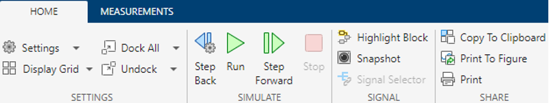
To launch the Style Settings side panel for the currently active scope, click Settings. In this panel, you can control settings related to the scope, including time and axes settings, display settings, style settings, and settings related to logging. For more information, see Settings in the Scope reference page.
To open a grid picker similar to the scope layout, click Display Grid. The layout can have a maximum of 16 rows and 16 columns.
If the number of displays is equal to the number of ports, signals from each port appear on separate displays. If the number of displays is less than the number of ports, signals from additional ports appear on the last display. For layouts with multiple columns and rows, ports are mapped down then across. If the number of displays is greater than the number of ports, the scope creates empty tiles.
Click Dock All to add all the opened scopes in the current model to the scope container. To automatically add newly opened scopes to the existing scope container, select Dock All > Dock New Scopes on Open.
Click Undock to remove the currently active scope from the container into a separate standalone window. When there are multiple scopes docked in the container, click Undock > Undock All to remove all scopes from the container into separate standalone windows.
The Measurements tab of the scope container has settings similar to the Measurements tab of the Scope block toolstrip.