Scope Bilevel Measurements

Bilevel Measurements

Display information about signal transitions, overshoots, undershoots, and cycles. To open the bilevel measurements panel:

• In the Measurements tab of the scope toolstrip, click Bilevel Settings () and select one or more of these drop-down options.

  • Transitions –– Transition measurements include the high and low state levels, rise time, fall time, and slew rate. When you select this parameter, transition measurements appear in the Transitions Pane.

  • Aberrations –– Aberration measurements include the preshoot, overshoot, undershoot, and settling time of the signal transitions. When you select this parameter, aberration measurements appear in the Aberrations Pane.

  • Cycles –– Cycle measurements include the pulse period, pulse width, and duty cycle. When you select this parameter, cycle measurements appear in the Cycles Pane.

State Level and Reference Level Settings

The state level and reference level settings enable you to modify the properties used to calculate various measurements involving transitions, overshoots, undershoots, and cycles. You can modify the high-state level, low-state level, state-level tolerance, upper-reference level, mid-reference level, and lower-reference level. To modify these properties, click Bilevel Settings > State Level or Bilevel Settings > Reference Level.

State Level Settings

• Auto State Level — When you select this parameter, the bilevel measurements panel detects the high- and low- state levels of a bilevel waveform. When you clear this parameter, you can enter in values for the high- and low- state levels manually.

  • High — Specify manually the value that denotes a positive polarity, or high-state level.

    

  • Low — Specify manually the value that denotes a negative polarity, or low-state level.

    

• State Level Tol. (%) — Tolerance within which the initial and final levels of each transition must be within their respective state levels. This value is expressed as a percentage of the difference between the high- and low-state levels.

Reference Level Settings

• Upper Ref. Level (%) — Compute the end of the rise-time measurement or the start of the fall time measurement using this parameter. This value is expressed as a percentage of the difference between the high- and low-state levels.

• Mid Ref. Level (%) — Determine when a transition occurs using this parameter. This value is expressed as a percentage of the difference between the high- and low- state levels. In the following figure, the mid-reference level is shown as the horizontal line, and its corresponding mid-reference level instant is shown as the vertical line.

  

• Lower Ref. Level (%) — Compute the end of the fall-time measurement or the start of the rise-time measurement using this parameter. This value is expressed as a percentage of the difference between the high- and low-state levels.

• Settle Seek (s) — The duration after the mid-reference level instant when each transition occurs used for computing a valid settling time. The settling time is displayed in the Aberrations pane.

  This value is equivalent to the settle-seek duration parameter d which you can set when you run the settlingtime function.

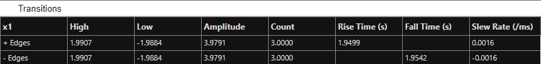
Transitions Pane

Display calculated measurements associated with the input signal changing between its two possible state level values, high and low. To enable this pane, select Bilevel Settings > Transitions.

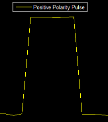
A positive-going transition, or rising edge, in a bilevel waveform is a transition from the low-state level to the high-state level. A positive-going transition has a slope value greater than zero. The following figure shows a positive-going transition.

When there is a plus sign (+) next to a text label, the measurement is a rising edge, a transition from a low-state level to a high-state level.

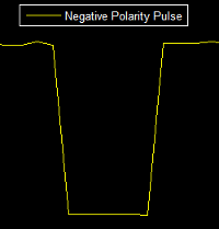
A negative-going transition, or falling edge, in a bilevel waveform is a transition from the high-state level to the low-state level. A negative-going transition has a slope value less than zero. The following figure shows a negative-going transition.

When there is a minus sign (–) next to a text label, the measurement is a falling edge, a transition from a high-state level to a low-state level.

The Transition measurements assume that the amplitude of the input signal is in units of volts. For the transition measurements to be valid, you must convert all input signals to volts.

• High — The high-amplitude state level of the input signal over the duration of the Time span parameter. You can set Time span parameter in the Scope tab > Settings > Time section.

• Low — The low-amplitude state level of the input signal over the duration of the Time span parameter. You can set Time span parameter in the Scope tab > Settings > Time section.

• Amplitude — Difference in amplitude between the high-state level and the low-state level.

• Count — The total number of positive- or negative- polarity edges counted within the displayed portion of the signal.

  • For + Edges, this value indicates the total number of positive-polarity, or rising edges counted.

  • For − Edges, this value indicates the total number of negative-polarity or falling edges counted.

• Rise Time (s) — Average amount of time required for each rising edge (+ Edges) to cross from the lower-reference level to the upper-reference level.

• Fall Time (s) — Average amount of time required for each falling edge (– Edges) to cross from the upper-reference level to the lower-reference level.

• Slew Rate (/ms) — The average slope of each rising-edge transition line and falling-edge transition line within the upper- and lower-percent reference levels in the displayed portion of the input signal.

  • For + Edges, this value indicates the average slope of each rising-edge transition line. The region in which the slew rate is calculated appears in gray in the following figure.

    

  • For − Edges, this value indicates the average slope of each falling edge transition line.

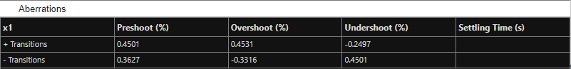
Aberrations Pane

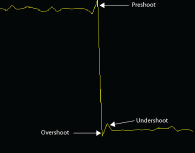
The Aberrations pane displays calculated measurements involving the distortion and damping of the input signal. Overshoot and undershoot refer to the amount that a signal respectively exceeds and falls below its final steady-state value. Preshoot refers to the amount before a transition that a signal varies from its initial steady-state value.

This figure shows preshoot, overshoot, and undershoot for a rising-edge transition (+ Transitions).

The next figure shows preshoot, overshoot, and undershoot for a falling-edge transition (− Transitions).

• Preshoot (%) — For + Transitions, this value indicates the average lowest aberration in the region immediately preceding each rising transition.

  For − Transitions, this value indicates the average highest aberration in the region immediately preceding each falling transition.

• Overshoot (%) — For + Transitions, this value indicates the average highest aberration in the region immediately following each rising transition.

  For − Transitions, this value indicates the average highest aberration in the region immediately following each falling transition.

• Undershoot (%) — For + Transitions, this value indicates the average lowest aberration in the region immediately following each rising transition.

  For − Transitions, this value indicates the average lowest aberration in the region immediately following each falling transition.

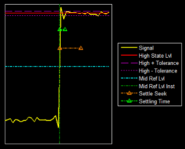
• Settling Time (s) — For + Transitions, this value indicates the average time required for each rising edge to enter and remain within the tolerance of the high-state level for the remainder of the settle-seek duration. The settling time in this case is the time after the mid-reference level instant when the signal crosses into and remains in the tolerance region around the high-state level. This crossing is illustrated in the following figure.

  

  For − Transitions, this value indicates the average time required for each falling edge to enter and remain within the tolerance of the low-state level for the remainder of the settle-seek duration. The settling time is the time after the mid-reference level instant when the signal crosses into and remains in the tolerance region around the low-state level.

  You can modify the settle-seek duration parameter in Bilevel Settings > Reference Level.

Cycles Pane

The Cycles pane displays calculated measurements pertaining to repetitions or trends in the displayed portion of the input signal.

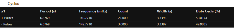
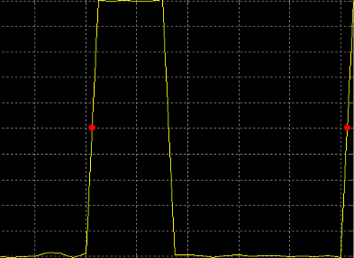
• Period (s) — Average duration between adjacent edges of identical polarity within the displayed portion of the input signal. The bilevel measurements panel calculates period as follows. It takes the difference between the mid-reference level instants of the initial transition of each positive-polarity pulse and the next positive-going transition. These mid-reference level instants appear as red dots in the following figure.

  

• Frequency — Reciprocal of the average period. Whereas period is typically measured in some metric form of seconds, or seconds per cycle, frequency is typically measured in Hz or cycles per second.

• Count — For + Pulses, this value indicates the number of positive-polarity pulses counted.

  For − Pulses, this value indicates the number of negative-polarity pulses counted.

• Width (s) — For + Pulses, this value indicates the average duration between rising and falling edges of each positive-polarity pulse within the displayed portion of the input signal.

  For − Pulses, this value indicates the average duration between rising and falling edges of each negative-polarity pulse within the displayed portion of the input signal.

• Duty Cycle (%) — For + Pulses, this value indicates the average ratio of pulse width to pulse period for each positive-polarity pulse within the displayed portion of the input signal.

  For − Pulses, this value indicates the average ratio of pulse width to pulse period for each negative-polarity pulse within the displayed portion of the input signal.

When you use the zoom options in the Scope, the bilevel measurements automatically adjust to the time range shown in the display. For example, you can zoom in on one rising edge to make the bilevel measurements panel display information about only that particular rising edge. However, this feature does not apply to the High and Low measurements.

Use Bilevel Measurements Panel with Clock Input Signal

This example shows how to use the Bilevel Measurements panel in the Time Scope block.

Open the example model ex-timescope-clockex:

open_system("ex_timescope_clockex")

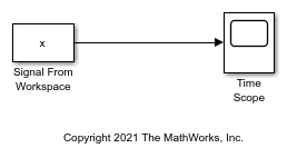
In this example, Simulink® imports the variable x , from the MATLAB® workspace. This variable is created when the model loads because the commands that construct it reside in the model Preload function. To view these commands,

1. On the Simulink toolbar, on the Modeling tab, in the Setup section, in the drop-down, select Model Properties.

2. In the Model Properties dialog box, select the Callbacks tab. The following lines of MATLAB code appear.

load clockex;
ts = t(2)-t(1);

Run your model and open the Time Scope block to see the time domain output.

To show the Bilevel Measurements panel, in the Measurements tab of the scope toolstrip, click Bilevel Settings and select Aberrations.

sim("ex_timescope_clockex")
open_system("ex_timescope_clockex/Time Scope")

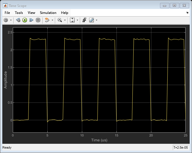
The value for the rising edge Settling Time parameter is not displayed because the default value of Settle Seek (s) is longer than the entire simulation.

Enter a smaller value of 2e-6 for Bilevel Settings > Reference Level > Settle Seek (s) parameter. The Time Scope now displays a rising edge settling time value of 118.392 ns.

The settling time value displayed is the statistical average of the settling times for all five rising edges.

To show the settling time for one rising edge, zoom in on that transition.

The Time Scope updates the rising edge settling time value to reflect the new time window.