Results for
Introduction
MCP is an open protocol that can link Claude and other AI Apps to MATLAB using MATLAB MCP Core Server (released in Nov 2025). For an introduction, see Exploring the MATLAB Model Context Protocol (MCP) Core Server with Claude Desktop. Here, I describe my experience with installation and testing Claude-Code and MATLAB, a security concern, and in particular how I "taught" Claude to handle various MATLAB file formats.
Setup
A basic installation requires you download for your operating system claude-code, matlab-mcp-core-server, and node.js. One configuration is a terminal-launched claude connected to MATLAB. To connect Claude App to MATLAB requires an alternate configuration step and I recommend it for interative use. The configuration defines the default node/folder and MATLAB APP location.
I recommend using Claude itself to guide you through the installation and configuration steps for your operating system by providing terminal commands. I append Claude’s general description of installation for my APPLE Silicon laptop. Once set up, just ask in Claude App to do something in MATLAB and MATLAB App will be launched.
Security warning: Explore the following at your own risk.
When working with Claude App, Claude code, and MATLAB, you are granting Claude AI access to read and write files. By default, you must approve (one time or forever) any action so you hopefully don’t clobber files etc. Claude App believes it can not directly access file outside the top node defined in the setup. For this reason, I set the top node to be a folder ..../Documents/MATLAB. However, Claude inherits MATLAB App's command line privileges, typically your full system privileges. Claude can describe for you some work-arounds like a Docker container which might still be license validation compatible. I have not explored such options. During my setup, Claude just provided me terminal commands to copy and run. After setup, I've demonstrated it can run system level commands via matlab:evaluate_matlab_code and the MCP server. Be careful out there!
My first test
Claude can write a text-based .m script, execute it, collect text standard output from it, and open files it makes (or any file). It cannot access figures that you might see in MATLAB App unless they are saved as files or embedded in files. As we will see, the figures generated by a Live Script are saved in an Claude-accessible format when the Live Script is saved so the code need not itself export them.
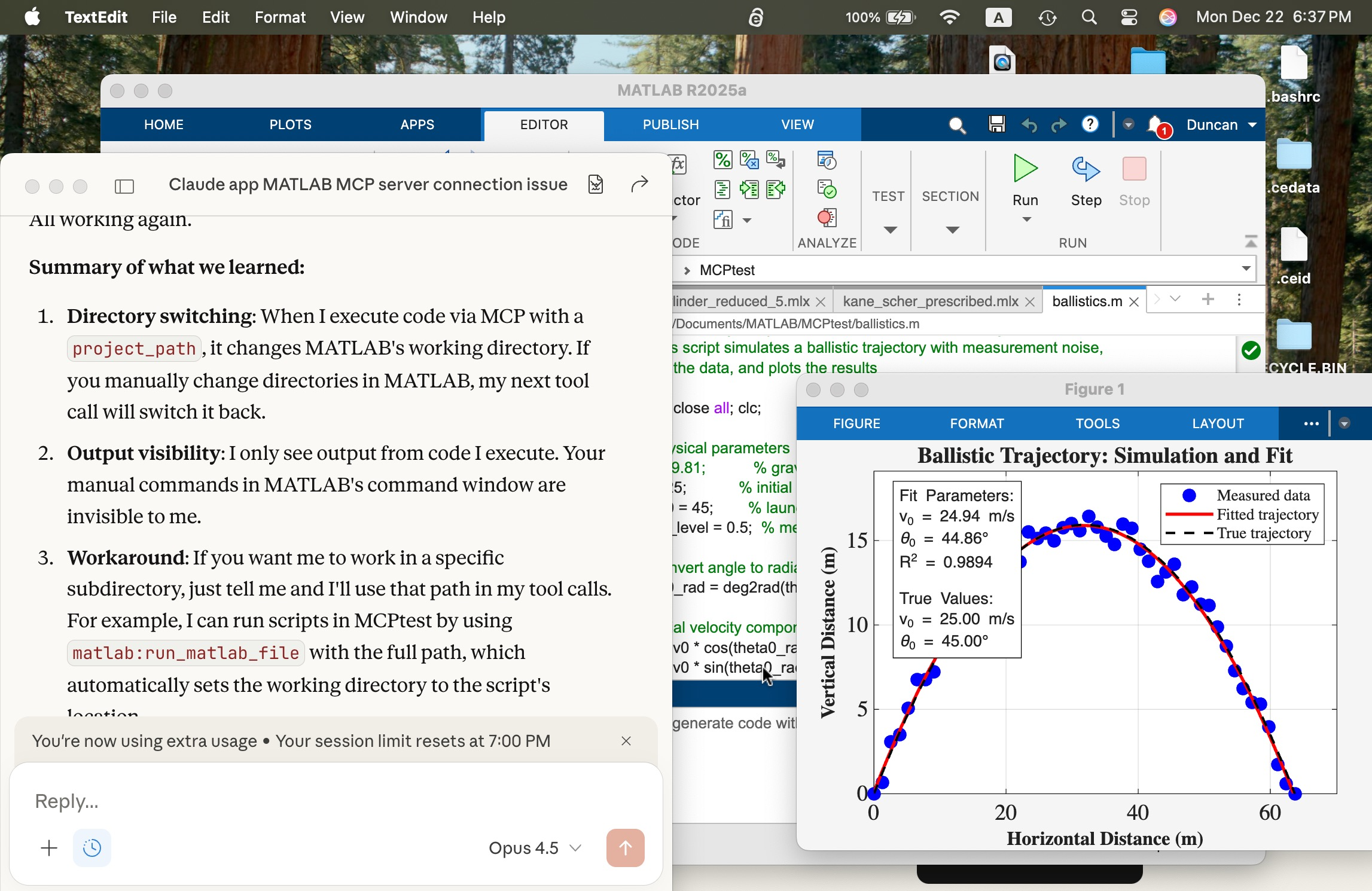
In the screen shot below, the window at left is the Claude App after a successful connection. The MATLAB App window shows a script in the MATLAB editor that simulates a ballistics experiment, the script created successfully with a terminal-interfaced Claude and a simple prompt on the first try.
I deliberately but trivially broke this script using MATLAB App interactively by commenting out a needed variable g (acceleration of gravity) and saving the script to the edit was accessible to Claude. Using Claude App after its connection, I fixed the script with a simple prompt and ran it successfully to make the figure you see. The visible MATLAB didn’t know the code had been altered and fixed by Claude until I reloaded the file. Claude recommends plots be saved in PNG or JPEG, not PDF. It can describe in detail a plot in a PNG and thusly judge if the code is functioning correctly.
Live Scripts with Claude
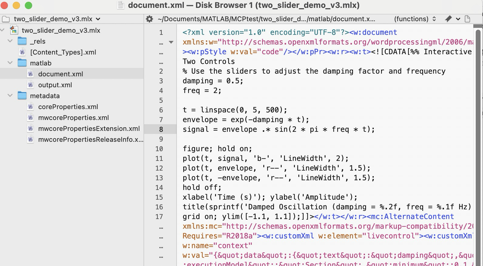
What about Live Scripts (.mlx) and the (2025a) .m live? A .mlx file is a zipped package of files mixing code and images wtih XML markup. You can peek inside one and edit it directly without unzipping and rezipping it using a tool like BBEdit on a Mac, as shown below. This short test script has two interactive slider controls. You can in v2025+ now save a .mlx in a transportable .m Live text file format. The .mlx and .m Live formats have special markup for formatted text, interactive features like sliders, and figures.
Claude can convert a vanilla .m file to .mlx using matlab.internal.liveeditor.openAndSave(source.m, dest.mlx) and the reverse matlab.internal.liveeditor.openAndConvert('myfile.mlx', 'myfile.m’).
These functions do not support .m Live yet apparently. It would be great if they did.
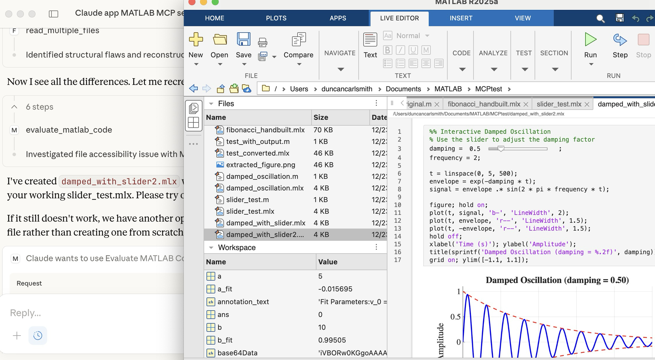
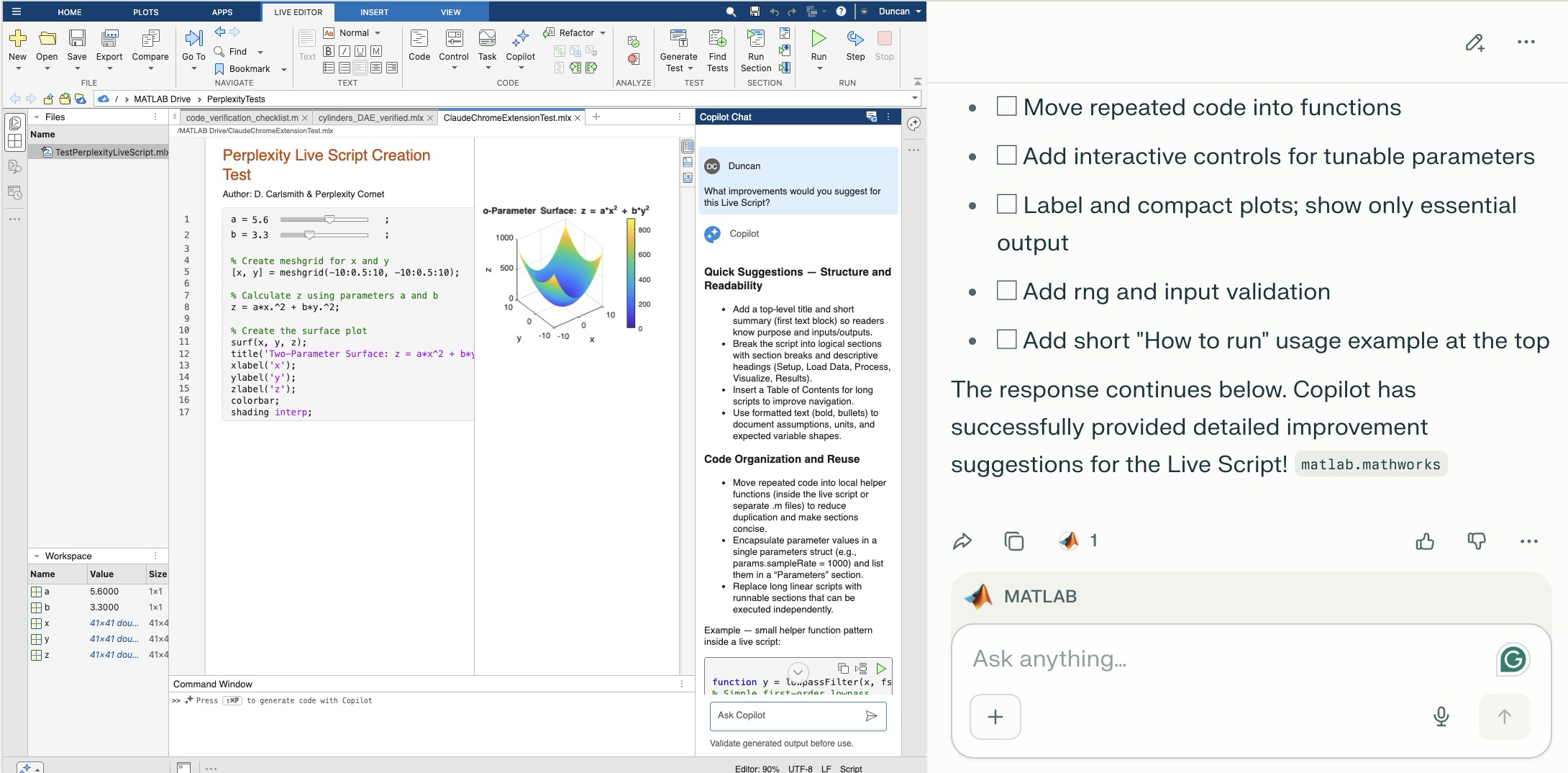
Vanilla Claude doesn’t know all the details of the .mlx and .m formats yet. To teach Claude these formats, I created a simple .mlx with interactive features (sliders), saved it, and exported it to .m Live. I then sketched for Claude these structures. Claude digested these files and was then able to create such formats from scratch immediately. Wow! In the figure below, you see Claude on the left after creating a .mlx with sliders from scratch. The successfully executed Live Script appears in the MATLAB App.
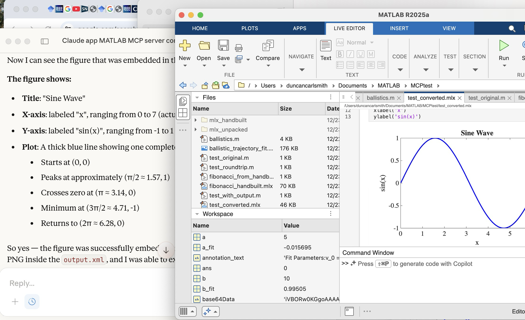
Once Claude knows the .mlx format, it can peek inside a saved .mlx, process a PNG figure saved there, and describe it, as illustrated below. Here you see Claude describing a plot it found in the .mlx shown in the MATLAB window.
Wrap up
This summarizes my first look at using claude-code. The generation of simple MATLAB codes with the latest models is increasingly trivial with Claude, Perplexity, Open.ai GPT and other apps and the direct method of code and other file transfer between a native MATLAB and Claude seems to beat a copy-paste workflow. New methods to connect MATLAB Online with commercial AI's like Comet and Anthropic's Chrome extension seem to me more fluid and intuitive in that the user and the AI are co-working the same interface without copy-paste steps, but seem slower.
Appendix
Here are installation and setup instructions for Mac from Claude for reference.
Setting Up Claude Code + MATLAB MCP Server on Mac
Part 1: Claude Code
Install via npm:
bash
npm install -g @anthropic-ai/claude-code
Or via Homebrew:
bash
brew install claude-code
Run it:
bash
cd /path/to/your/project
claude
You'll need to authenticate with your Anthropic account on first run. Claude Code works in your terminal and can read/write files, run commands, and do agentic coding tasks.
Part 2: MATLAB MCP Server
Step 1: Download the server binary
Go to the MathWorks GitHub or File Exchange and download matlab-mcp-core-server for macOS (Apple Silicon or Intel depending on your Mac).
Step 2: Make it executable
bash
chmod +x ~/Downloads/matlab-mcp-core-server
Step 3: Create/edit Claude Desktop config
Edit ~/Library/Application Support/Claude/claude_desktop_config.json:
json
{
"mcpServers": {
"matlab": {
"command": "/Users/YOURUSERNAME/Downloads/matlab-mcp-core-server",
"args": ["--matlab-root", "/Applications/MATLAB_R2025a.app"]
},
"filesystem": {
"command": "npx",
"args": [
"@modelcontextprotocol/server-filesystem",
"/Users/YOURUSERNAME/Documents/MATLAB"
]
}
}
}
Replace YOURUSERNAME with your actual username, and adjust the MATLAB version if needed.
Step 4: Install Node.js (if not already)
bash
brew install node
Step 5: Restart Claude Desktop
Quit fully (Cmd+Q) and reopen. You should see a hammer/tools icon indicating MCP servers are connected.
Part 3: Verify Connection
In Claude Desktop, ask me to run MATLAB code. I should be able to execute:
matlab
disp('Hello from MATLAB!')
Troubleshooting
Check logs:
bash
cat ~/Library/Logs/Claude/mcp-server-matlab.log
cat ~/Library/Logs/Claude/mcp.log
Common issues:
- Missing --matlab-root argument → "no valid MATLAB environments found"
Connecting Claude App to MATLAB via MCP Server
Edit ~/Library/Application Support/Claude/claude_desktop_config.json:
json
{
"mcpServers": {
"filesystem": {
"command": "npx",
"args": [
"-y",
"@modelcontextprotocol/server-filesystem",
"/Users/YOURUSERNAME/Documents/MATLAB"
]
},
"matlab": {
"command": "/Users/YOURUSERNAME/Downloads/matlab-mcp-core-server",
"args": [
"--matlab-root", "/Applications/MATLAB_R2025a.app"
]
}
}
}
Then fully quit Claude Desktop (Cmd+Q) and reopen.
Comet browser can figure out and operate a user interface on the web including MATLAB Online. The screen shot shows MATLAB online to the left of the Comet AI. You see a test Live Script with sliders thjat Comet created in a folder (that it created). Comet is summarizing suggested improvements it requested of MATLAB Online's Copilot. Comet can plow into the arcane NASA astrophysical database interface SIMBAD, figure out how to grab information about, say, a star orbiting the black hole in the center of our galaxy and structure that information into a MATLAB data structure in a MATLAB script and run the script in MATLAB Online and display the results in the structure - it succeeded on the first try. It can do a Google Scholar citation tree search and park the results in MATLAB (success first try) or presumably in say MS Word in Office online. Presumably it can switch to a JuypterHub tab to then run a notebook or what you will. It can make mistakes, explore and discover GUI options, and recover e.g. use undo paste in MATLAB, operate in the command window, get help via the GUI if needed. Not at light speed but this seems enabling. Just released, Claude Chrome Extension Beta has similar capabilities.
Inspired in part by Christmas Trees, I'm curious about people's experience using AI to generate Matlab code.
1. Do you use AI to generate production code or just for experimentation/fun code?
2. Do you use the AI for a complete solution? Or is it more that the AI gets you most of the way there and you have to apply the finishing touches manually?
3. What level of quality would you consider the generated code? Does it follow "standard" Matlab coding practices? Is it well commented? Factored into modular functions? Argument checking? Memory efficient? Fast execution? Etc.?
4. Does the AI ever come up with a good or clever solution of which you wouldn't have thought or maybe of which you weren't even aware?
5. Is it easy/hard to express your requirements in a manner that the AI tool effectively translates into something useful?
6. Any other thoughts you'd care to share?
I thought it would be fun to vibe code Christmas trees.
Model: Claude Sonnet4.5
Prompt: Write a MATLAB script that draws a Christmas tree. There should be decorations and presents too.
Result:
christmasTree()

function christmasTree()
% Christmas Tree with Decorations and Presents
% Creates a festive scene with a decorated tree and gift boxes
figure('Color', 'w', 'Position', [100, 100, 800, 900]);
hold on;
axis equal;
axis off;
xlim([-3, 3]);
ylim([0, 10]);
% Draw the tree (three layered triangular sections)
drawTreeSection(0, 2, 2.5, 2.5, [0.1, 0.5, 0.1]);
drawTreeSection(0, 3.5, 2, 2, [0.15, 0.55, 0.15]);
drawTreeSection(0, 4.8, 1.5, 1.8, [0.2, 0.6, 0.2]);
% Tree trunk
rectangle('Position', [-0.3, 0, 0.6, 2], 'FaceColor', [0.4, 0.2, 0.1], ...
'EdgeColor', 'none');
% Add decorations
addOrnaments();
addTinsel();
% Star on top
drawStar(0, 7.2, 0.4, [1, 0.84, 0]);
% Add presents under the tree
drawPresent(-1.8, 0, 0.6, 0.5, [0.8, 0.1, 0.1], [1, 0.84, 0]);
drawPresent(-0.8, 0, 0.5, 0.6, [0.1, 0.3, 0.8], [0.9, 0.9, 0.9]);
drawPresent(1.2, 0, 0.7, 0.4, [0.7, 0.5, 0.9], [0.2, 0.8, 0.2]);
drawPresent(0.2, 0, 0.4, 0.5, [1, 0.7, 0.1], [0.8, 0.1, 0.1]);
% Add some snow on the ground
scatter(randn(1, 100)*2.5, rand(1, 100)*0.3, 20, 'w', 'filled', ...
'MarkerEdgeColor', [0.8, 0.8, 0.8]);
title('Merry Christmas!', 'FontSize', 24, 'Color', [0.8, 0.1, 0.1], ...
'FontWeight', 'bold');
hold off;
end
function drawTreeSection(x, y, width, height, color)
% Draw a triangular section of the tree
xPoints = [x - width, x + width, x];
yPoints = [y, y, y + height];
fill(xPoints, yPoints, color, 'EdgeColor', [0.05, 0.3, 0.05], ...
'LineWidth', 1.5);
end
function addOrnaments()
% Add colorful baubles to the tree
ornamentColors = [
1, 0, 0; % Red
0, 0, 1; % Blue
1, 0.84, 0; % Gold
0.9, 0.1, 0.5;% Pink
0.5, 0, 0.5 % Purple
];
% Ornament positions (x, y coordinates)
positions = [
-1.5, 2.5; 1.5, 2.5; 0, 3.2;
-1.2, 3.8; 1.2, 3.8; -0.6, 4.2; 0.6, 4.2;
-0.8, 5.2; 0.8, 5.2; 0, 5.8; -0.4, 6.3; 0.4, 6.3
];
for i = 1:size(positions, 1)
colorIdx = mod(i-1, size(ornamentColors, 1)) + 1;
x = positions(i, 1);
y = positions(i, 2);
% Draw bauble
theta = linspace(0, 2*pi, 50);
radius = 0.15;
xCirc = x + radius * cos(theta);
yCirc = y + radius * sin(theta);
fill(xCirc, yCirc, ornamentColors(colorIdx, :), ...
'EdgeColor', ornamentColors(colorIdx, :)*0.7, 'LineWidth', 1.5);
% Add highlight for shine
highlightX = x - radius*0.4 + radius*0.3*cos(theta(1:15));
highlightY = y + radius*0.4 + radius*0.3*sin(theta(1:15));
fill(highlightX, highlightY, [1, 1, 1], 'EdgeColor', 'none', ...
'FaceAlpha', 0.6);
end
end
function addTinsel()
% Add sparkly tinsel effect
tinselX = [-1.8, -1.2, -0.5, 0.2, 0.9, 1.6];
tinselY = [2.8, 3.5, 4.0, 4.5, 5.0, 5.5];
for i = 1:length(tinselX)
plot(tinselX(i) + randn(1, 5)*0.1, tinselY(i) + rand(1, 5)*0.2, ...
'*', 'Color', [1, 0.84, 0], 'MarkerSize', 8, 'LineWidth', 1.5);
end
end
function drawStar(x, y, size, color)
% Draw a 5-pointed star on top of the tree
angles = linspace(0, 2*pi, 11);
radii = repmat([size, size*0.4], 1, 5);
radii = [radii, radii(1)];
xStar = x + radii .* cos(angles - pi/2);
yStar = y + radii .* sin(angles - pi/2);
fill(xStar, yStar, color, 'EdgeColor', [0.8, 0.6, 0], 'LineWidth', 2);
% Add sparkle
plot(x, y, '*', 'Color', [1, 1, 1], 'MarkerSize', 15, 'LineWidth', 2);
end
function drawPresent(x, y, width, height, boxColor, ribbonColor)
% Draw a gift box with ribbon and bow
% Box
rectangle('Position', [x, y, width, height], 'FaceColor', boxColor, ...
'EdgeColor', boxColor*0.7, 'LineWidth', 2);
% Vertical ribbon
ribbonWidth = width * 0.15;
rectangle('Position', [x + width/2 - ribbonWidth/2, y, ribbonWidth, height], ...
'FaceColor', ribbonColor, 'EdgeColor', 'none');
% Horizontal ribbon
ribbonHeight = height * 0.15;
rectangle('Position', [x, y + height/2 - ribbonHeight/2, width, ribbonHeight], ...
'FaceColor', ribbonColor, 'EdgeColor', 'none');
% Bow on top
bowX = x + width/2;
bowY = y + height;
bowSize = width * 0.2;
% Left loop
theta = linspace(0, pi, 30);
fill(bowX - bowSize*0.3 + bowSize*0.5*cos(theta), ...
bowY + bowSize*0.5*sin(theta), ribbonColor, 'EdgeColor', 'none');
% Right loop
fill(bowX + bowSize*0.3 + bowSize*0.5*cos(theta), ...
bowY + bowSize*0.5*sin(theta), ribbonColor, 'EdgeColor', 'none');
% Center knot
theta = linspace(0, 2*pi, 30);
fill(bowX + bowSize*0.25*cos(theta), bowY + bowSize*0.25*sin(theta), ...
ribbonColor*0.8, 'EdgeColor', 'none');
end
I like this quote, what do you think?
"If the part of programming you enjoy most is the physical act of writing code, then agents will feel beside the point. You’re already where you want to be, even just with some Copilot or Cursor-style intelligent code auto completion, which makes you faster while still leaving you fully in the driver’s seat about the code that gets written.
But if the part you care about is the decision-making around the code, agents feel like they clear space. They take care of the mechanical expression and leave you with judgment, tradeoffs, and intent. Because truly, for someone at my experience level, that is my core value offering anyway. When I spend time actually typing code these days with my own fingers, it feels like a waste of my time."
— Obie Fernandez, What happens when the coding becomes the least interesting part of the work
Hi everyone
I've been using ThingSpeak for several years now without an issue until last Thursday.
I have four ThingSpeak channels which are used by three Arduino devices (in two locations/on two distinct networks) all running the same code.
All three devices stopped being able to write data to my ThingSpeak channels around 17:00 CET on 4 Dec and are still unable to.
Nothing changed on this side, let alone something that would explain the problem.
I would note that data can still be written to all the channels via a browser so there is no fundamental problem with the channels (such as being full).
Since the above date and time, any HTTP/1.1 'update' (write) requests via the REST API (using both simple one-write GET requests or bulk JSON POST requests) are timing out after 5 seconds and no data is being written. The 5 second timeout is my Arduino code's default, but even increasing it to 30 seconds makes no difference. Before all this, responses from ThingSpeak were sub-second.
I have recompiled the Arduino code using the latest libraries and that didn't help.
I have tested the same code again another random api (api.ipify.org) and that works just fine.
Curl works just fine too, also usng HTTP/1.1
So the issue appears to be something particular to the combination of my Arduino code *and* the ThingSpeak environment, where something changed on the ThingSpeak end at the above date and time.
If anyone in the community has any suggestions as to what might be going on, I would greatly appreciate the help.
Peter
In a recent blog post, @Guy Rouleau writes about the new Simulink Copilot Beta. Sign ups are on the Copilot Beta page below. Let him know what you think.
Guy's Blog Post - https://blogs.mathworks.com/simulink/2025/12/01/a-copilot-for-simulink/
Simulink Copilot Beta - https://www.mathworks.com/products/simulink-copilot.html
If you haven't solved the problem yet, below hints guide how the algorithm should be implemented and clarify subtle rules that are easy to miss.
1. Shield is ONLY defended in HOME matches of the CURRENT holder - Even if a team beats the Shield holder in an away match, that does NOT count as a Shield defense.
2. A team defends the Shield ONLY when:
> They currently hold it.
> They are home team in that match
3. Shield transfer happens ONLY if the HOLDER plays a home match AND loses - A team may lose an away match — no effect.
4. The output ALWAYS includes the initial holder as the first row.
5. Defenses count resets for each new holder. - Every holder accumulates their own count until they lose it at home.
6. Match numbers are 1-indexed in the input, but “0” is used for initial state - The first real match is Match 1, but the output starts with Match 0.
7. Output row is created ONLY WHEN SHIELD CHANGES HANDS - This is an important hidden detail. A new row is appended, When the current holder loses a home match → Shield taken by visitor. If no loss at home occurs after that → no new row until next change.
8. The last holder’s defense count goes until the season ends - Even if they lose away later.
9. If a holder never gets a home match, defenses = 0.
10. In case the holder loses their very first home match → defenses = 0.
11. Shield changes only on HOME LOSS, not on a draw.
I hope above hints will help you in solving the problem.
Thanks and Regards,
Dev

% Recreation of Saturn photo
figure('Color', 'k', 'Position', [100, 100, 800, 800]);
ax = axes('Color', 'k', 'XColor', 'none', 'YColor', 'none', 'ZColor', 'none');
hold on;
% Create the planet sphere
[x, y, z] = sphere(150);
% Saturn colors - pale yellow/cream gradient
saturn_radius = 1;
% Create color data based on latitude for gradient effect
lat = asin(z);
color_data = rescale(lat, 0.3, 0.9);
% Plot Saturn with smooth shading
planet = surf(x*saturn_radius, y*saturn_radius, z*saturn_radius, ...
color_data, ...
'EdgeColor', 'none', ...
'FaceColor', 'interp', ...
'FaceLighting', 'gouraud', ...
'AmbientStrength', 0.3, ...
'DiffuseStrength', 0.6, ...
'SpecularStrength', 0.1);
% Use a cream/pale yellow colormap for Saturn
cream_map = [linspace(0.4, 0.95, 256)', ...
linspace(0.35, 0.9, 256)', ...
linspace(0.2, 0.7, 256)'];
colormap(cream_map);
% Create the ring system
n_points = 300;
theta = linspace(0, 2*pi, n_points);
% Define ring structure (inner radius, outer radius, brightness)
rings = [
1.2, 1.4, 0.7; % Inner ring
1.45, 1.65, 0.8; % A ring
1.7, 1.85, 0.5; % Cassini division (darker)
1.9, 2.3, 0.9; % B ring (brightest)
2.35, 2.5, 0.6; % C ring
2.55, 2.8, 0.4; % Outer rings (fainter)
];
% Create rings as patches
for i = 1:size(rings, 1)
r_inner = rings(i, 1);
r_outer = rings(i, 2);
brightness = rings(i, 3);
% Create ring coordinates
x_inner = r_inner * cos(theta);
y_inner = r_inner * sin(theta);
x_outer = r_outer * cos(theta);
y_outer = r_outer * sin(theta);
% Front side of rings
ring_x = [x_inner, fliplr(x_outer)];
ring_y = [y_inner, fliplr(y_outer)];
ring_z = zeros(size(ring_x));
% Color based on brightness
ring_color = brightness * [0.9, 0.85, 0.7];
fill3(ring_x, ring_y, ring_z, ring_color, ...
'EdgeColor', 'none', ...
'FaceAlpha', 0.7, ...
'FaceLighting', 'gouraud', ...
'AmbientStrength', 0.5);
end
% Add some texture/gaps in the rings using scatter
n_particles = 3000;
r_particles = 1.2 + rand(1, n_particles) * 1.6;
theta_particles = rand(1, n_particles) * 2 * pi;
x_particles = r_particles .* cos(theta_particles);
y_particles = r_particles .* sin(theta_particles);
z_particles = (rand(1, n_particles) - 0.5) * 0.02;
% Vary particle brightness
particle_colors = repmat([0.8, 0.75, 0.6], n_particles, 1) .* ...
(0.5 + 0.5*rand(n_particles, 1));
scatter3(x_particles, y_particles, z_particles, 1, particle_colors, ...
'filled', 'MarkerFaceAlpha', 0.3);
% Add dramatic outer halo effect - multiple layers extending far out
n_glow = 20;
for i = 1:n_glow
glow_radius = 1 + i*0.35; % Extend much farther
alpha_val = 0.08 / sqrt(i); % More visible, slower falloff
% Color gradient from cream to blue/purple at outer edges
if i <= 8
glow_color = [0.9, 0.85, 0.7]; % Warm cream/yellow
else
% Gradually shift to cooler colors
mix = (i - 8) / (n_glow - 8);
glow_color = (1-mix)*[0.9, 0.85, 0.7] + mix*[0.6, 0.65, 0.85];
end
surf(x*glow_radius, y*glow_radius, z*glow_radius, ...
ones(size(x)), ...
'EdgeColor', 'none', ...
'FaceColor', glow_color, ...
'FaceAlpha', alpha_val, ...
'FaceLighting', 'none');
end
% Add extensive glow to rings - make it much more dramatic
n_ring_glow = 12;
for i = 1:n_ring_glow
glow_scale = 1 + i*0.15; % Extend farther
alpha_ring = 0.12 / sqrt(i); % More visible
for j = 1:size(rings, 1)
r_inner = rings(j, 1) * glow_scale;
r_outer = rings(j, 2) * glow_scale;
brightness = rings(j, 3) * 0.5 / sqrt(i);
x_inner = r_inner * cos(theta);
y_inner = r_inner * sin(theta);
x_outer = r_outer * cos(theta);
y_outer = r_outer * sin(theta);
ring_x = [x_inner, fliplr(x_outer)];
ring_y = [y_inner, fliplr(y_outer)];
ring_z = zeros(size(ring_x));
% Color gradient for ring glow
if i <= 6
ring_color = brightness * [0.9, 0.85, 0.7];
else
mix = (i - 6) / (n_ring_glow - 6);
ring_color = brightness * ((1-mix)*[0.9, 0.85, 0.7] + mix*[0.65, 0.7, 0.9]);
end
fill3(ring_x, ring_y, ring_z, ring_color, ...
'EdgeColor', 'none', ...
'FaceAlpha', alpha_ring, ...
'FaceLighting', 'none');
end
end
% Add diffuse glow particles for atmospheric effect
n_glow_particles = 8000;
glow_radius_particles = 1.5 + rand(1, n_glow_particles) * 5;
theta_glow = rand(1, n_glow_particles) * 2 * pi;
phi_glow = acos(2*rand(1, n_glow_particles) - 1);
x_glow = glow_radius_particles .* sin(phi_glow) .* cos(theta_glow);
y_glow = glow_radius_particles .* sin(phi_glow) .* sin(theta_glow);
z_glow = glow_radius_particles .* cos(phi_glow);
% Color particles based on distance - cooler colors farther out
particle_glow_colors = zeros(n_glow_particles, 3);
for i = 1:n_glow_particles
dist = glow_radius_particles(i);
if dist < 3
particle_glow_colors(i,:) = [0.9, 0.85, 0.7];
else
mix = (dist - 3) / 4;
particle_glow_colors(i,:) = (1-mix)*[0.9, 0.85, 0.7] + mix*[0.5, 0.6, 0.9];
end
end
scatter3(x_glow, y_glow, z_glow, rand(1, n_glow_particles)*2+0.5, ...
particle_glow_colors, 'filled', 'MarkerFaceAlpha', 0.05);
% Lighting setup
light('Position', [-3, -2, 4], 'Style', 'infinite', ...
'Color', [1, 1, 0.95]);
light('Position', [2, 3, 2], 'Style', 'infinite', ...
'Color', [0.3, 0.3, 0.4]);
% Camera and view settings
axis equal off;
view([-35, 25]); % Angle to match saturn_photo.jpg - more dramatic tilt
camva(10); % Field of view - slightly wider to show full halo
xlim([-8, 8]); % Expanded to show outer halo
ylim([-8, 8]);
zlim([-8, 8]);
% Material properties
material dull;
title('Saturn - Left click: Rotate | Right click: Pan | Scroll: Zoom', 'Color', 'w', 'FontSize', 12);
% Enable interactive camera controls
cameratoolbar('Show');
cameratoolbar('SetMode', 'orbit'); % Start in rotation mode

% Custom mouse controls
set(gcf, 'WindowButtonDownFcn', @mouseDown);
function mouseDown(src, ~)
selType = get(src, 'SelectionType');
switch selType
case 'normal' % Left click - rotate
cameratoolbar('SetMode', 'orbit');
rotate3d on;
case 'alt' % Right click - pan
cameratoolbar('SetMode', 'pan');
pan on;
end
end
Hello,
I have Arduino DIY Geiger Counter, that uploads data to my channel here in ThingSpeak (3171809), using ESP8266 WiFi board. It sends CPM values (counts per minute), Dose, VCC and Max CPM for 24h. They are assignet to Field from 1 to 4 respectively. How can I duplicate Field 1, so I could create different time chart for the same measured unit? Or should I duplicate Field 1 chart, and how? I tried to find the answer here in the blog, but I couldn't.

I have to say that I'm not an engineer or coder, just can simply load some Arduino sketches and few more things, so I'll be very thankfull if someone could explain like for non-IT users.
Regards,
Emo
Many MATLAB Cody problems involve solving congruences, modular inverses, Diophantine equations, or simplifying ratios under constraints. A powerful tool for these tasks is the Extended Euclidean Algorithm (EEA), which not only computes the greatest common divisor, gcd(a,b), but also provides integers x and y such that: a*x + b*y = gcd(a,b) - which is Bezout's identity.
Use of the Extended Euclidean Algorithm is very using in solving many different types of MATLAB Cody problems such as:
- Computing modular inverses safely, even for very large numbers
- Solving linear Diophantine equations
- Simplifing fractions or finding nteger coefficients without using symbolic tools
- Avoiding loops (EEA can be implemented recursively)
Below is a recursive implementation of the EEA.
function [g,x,y] = egcd(a,b)
% a*x + b*y = g [gcd(a,b)]
if b == 0
g = a; x = 1; y = 0;
else
[g, x1, y1] = egcd(b, mod(a,b));
x = y1;
y = x1 - floor(a/b)*y1;
end
end
Problem:
Given integers a and m, return the modular inverse of a (mod m).
If the inverse does not exist, return -1.
function inv = modInverse(a,m)
[g,x,~] = egcd(a,m);
if g ~= 1 % inverse doesn't exist
inv = -1;
else
inv = mod(x,m); % Bézout coefficient gives the inverse
end
end
%find the modular inverse of 19 (mod 5)
inv=modInverse(19,5)
Congratulations to all the Relentless Coders who have completed the problem set. I hope you weren't too busy relentlessly solving problems to enjoy the silliness I put into them.
If you've solved the whole problem set, don't forget to help out your teammates with suggestions, tips, tricks, etc. But also, just for fun, I'm curious to see which of my many in-jokes and nerdy references you noticed. Many of the problems were inspired by things in the real world, then ported over into the chaotic fantasy world of Nedland.
I guess I'll start with the obvious real-world reference: @Ned Gulley (I make no comment about his role as insane despot in any universe, real or otherwise.)
Hi Everyone!
As this is the most difficult question in problem group "Cody Contest 2025". To solve this problem, It is very important to understand all the hidden clues in the problem statement. Because everything is not directly visible.
For those who tried the problem, but were not able to solve. You might have missed any of the below hints -
- “The other players do not get to see which card has been shown, but they do know which three cards were asked for and that the player asked had one of them.” - Even when the card identity isn’t revealed (result = 0), you still gain partial knowledge — the asked player must have at least one of those three cards, meaning you can mark other players as not having all three simultaneously.
- "If it is your turn, you know the exact identity of that card" - You only know the exact shown card when result = 1, 2, or 3 — and it must be your turn. If someone else asked (even if you know result = 0), you don’t know which one was shown. So the meaning of result depends on whose turn it was, which is implicit — MATLAB code must assume that turns alternate 1→m→1, so your turn index is determined by (t-1) mod m + 1 == pnum.
- "Any leftover cards are placed face-up so that all players can see them" - These cards (commoncards) are not in anyone’s hand and cannot be in the envelope. So they’re not just visible — they’re logical constraints to eliminate from deduction.
- “It may be possible to determine the solution from less information than is given, but the information given will always be sufficient.”
- "Turn order is implied, not given explicitly" - Players take turns in order (1 to m, and back to 1).
On considering all the clues and constraints in the question, you will definitely be able to card for each category present in envelope.
I hope above clues will be useful for you.
Thank you, wishing you the success!
Regards,
Dev
Experimenting with Agentic AI
44%
I am an AI skeptic
0%
AI is banned at work
11%
I am happy with Conversational AI
44%
9 votes
When solving Cody problems, sometimes your solution takes too long — especially if you’re recomputing large arrays or iterative sequences every time your function is called.
The Cody work area resets between separate runs of your code, but within one Cody test suite, your function may be called multiple times in a single session.
This is where persistent variables come in handy.
A persistent variable keeps its value between function calls, but only while MATLAB is still running your function suite.
This means:
- You can cache results to avoid recomputation.
- You can accumulate data across multiple calls.
- But it resets when Cody or MATLAB restarts.
Suppose you’re asked to find the n-th Fibonacci number efficiently — Cody may time out if you use recursion naively. Here’s how to use persistent to store computed values:
function f = fibPersistent(n)
import java.math.BigInteger
persistent F
if isempty(F)
F=[BigInteger('0'),BigInteger('1')];
for k=3:10000
F(k)=F(k-1).add(F(k-2));
end
end
% Extend the stored sequence only if needed
while length(F) <= n
F(end+1)=F(end).add(F(end-1));
end
f = char(F(n+1).toString); % since F(1) is really F(0)
end
%calling function 100 times
K=arrayfun(@(x)fibPersistent(x),randi(10000,1,100),'UniformOutput',false);
K(100)
The fzero function can handle extremely messy equations — even those mixing exponentials, trigonometric, and logarithmic terms — provided the function is continuous near the root and you give a reasonable starting point or interval.
It’s ideal for cases like:
- Solving energy balance equations
- Finding intersection points of nonlinear models
- Determining parameters from experimental data
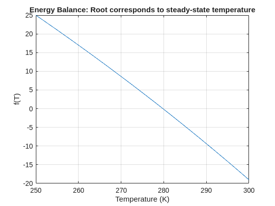
Example: Solving for Equilibrium Temperature in a Heat Radiation-Conduction Model
Suppose a spacecraft component exchanges heat via conduction and radiation with its environment. At steady state, the power generated internally equals the heat lost:
Given constants:
 = 25 W
- k = 0.5 W/K
- ϵ = 0.8
- σ = 5.67e−8 W/m²K⁴
- A = 0.1 m²
 = 250 K
Find the steady-state temperature, T.
% Given constants
Qgen = 25;
k = 0.5;
eps = 0.8;
sigma = 5.67e-8;
A = 0.1;
Tinf = 250;
% Define the energy balance equation (set equal to zero)
f = @(T) Qgen - (k*(T - Tinf) + eps*sigma*A*(T.^4 - Tinf^4));
% Plot for a sense of where the root lies before implementing
fplot(f, [250 300]); grid on
xlabel('Temperature (K)'); ylabel('f(T)')
title('Energy Balance: Root corresponds to steady-state temperature')
% Use fzero with an interval that brackets the root
T_eq = fzero(f, [250 300]);
fprintf('Steady-state temperature: %.2f K\n', T_eq);
I set my 3D matrix up with the players in the 3rd dimension. I set up the matrix with: 1) player does not hold the card (-1), player holds the card (1), and unknown holding the card (0). I moved through the turns (-1 and 1) that are fixed first. Then cycled through the conditional turns (0) while checking the cards of each player using the hints provided until it was solved. The key for me in solving several of the tests (11, 17, and 19) was looking at the 1's and 0's being held by each player.
sum(cardState==1,3);%any zeros in this 2D matrix indicate possible cards in the solution
sum(cardState==0,3)>0;%the ones in this 2D matrix indicate the only unknown positions
sum(cardState==1,3)|sum(cardState==0,3)>0;%oring the two together could provide valuable information
Some MATLAB Cody problems prohibit loops (for, while) or conditionals (if, switch, while), forcing creative solutions.
One elegant trick is to use nested functions and recursion to achieve the same logic — while staying within the rules.
Example: Recursive Summation Without Loops or Conditionals
Suppose loops and conditionals are banned, but you need to compute the sum of numbers from 1 to n. This is a simple example and obvisously n*(n+1)/2 would be preferred.
function s = sumRecursive(n)
zero=@(x)0;
s = helper(n); % call nested recursive function
function out = helper(k)
L={zero,@helper};
out = k+L{(k>0)+1}(k-1);
end
end
sumRecursive(10)
- The helper function calls itself until the base case is reached.
- Logical indexing into a cell array (k>0) act as an 'if' replacement.
- MATLAB allows nested functions to share variables and functions (zero), so you can keep state across calls.
Tips:
- Replace 'if' with logical indexing into a cell array.
- Replace for/while with recursion.
- Nested functions are local and can access outer variables, avoiding global state.
Many MATLAB Cody problems involve recognizing integer sequences.
If a sequence looks familiar but you can’t quite place it, the On-Line Encyclopedia of Integer Sequences (OEIS) can be your best friend.
OEIS will often identify the sequence, provide a formula, recurrence relation, or even direct MATLAB-compatible pseudocode.
Example: Recognizing a Cody Sequence
Suppose you encounter this sequence in a Cody problem:
1, 1, 2, 3, 5, 8, 13, 21, ...
Entering it on OEIS yields A000045 – The Fibonacci Numbers, defined by:
F(n) = F(n-1) + F(n-2), with F(1)=1, F(2)=1
You can then directly implement it in MATLAB:
function F = fibSeq(n)
F = zeros(1,n);
F(1:2) = 1;
for k = 3:n
F(k) = F(k-1) + F(k-2);
end
end
fibSeq(15)
When solving MATLAB Cody problems involving very large integers (e.g., factorials, Fibonacci numbers, or modular arithmetic), you might exceed MATLAB’s built-in numeric limits.
To overcome this, you can use Java’s java.math.BigInteger directly within MATLAB — it’s fast, exact, and often accepted by Cody if you convert the final result to a numeric or string form.
Below is an example of using it to find large factorials.
function s = bigFactorial(n)
import java.math.BigInteger
f = BigInteger('1');
for k = 2:n
f = f.multiply(BigInteger(num2str(k)));
end
s = char(f.toString); % Return as string to avoid overflow
end
bigFactorial(100)