Wavelet Time-Frequency Analyzer
Description
The Wavelet Time-Frequency Analyzer app is an interactive tool for visualizing scalograms of real- and complex-valued 1-D signals. The scalogram is the absolute value of the continuous wavelet transform (CWT) plotted as a function of time and frequency. Frequency is plotted on a logarithmic scale. With the app, you can:
Access all 1-D signals in your MATLAB® workspace
Import multiple signals simultaneously
Adjust default parameters and visualize scalograms using
cwtSelect desired analytic wavelet
Adjust analytic Morse wavelet symmetry and time-bandwidth parameters
Export the CWT to your workspace
Recreate the scalogram in your workspace by generating a MATLAB script
For more information, see Using Wavelet Time-Frequency Analyzer App.
Open the Wavelet Time-Frequency Analyzer App
MATLAB Toolstrip: On the Apps tab, under Signal Processing and Audio, click the app icon.
MATLAB command prompt: Enter
waveletTimeFrequencyAnalyzer.
Examples
Load three 1-D signals into the MATLAB® workspace: an electrocardiogram signal, a hyperbolic chirp signal, and the NPG2006 dataset.
load wecg
load hyperbolchirp
load npg2006
Extract the complex-valued signal from the npg2006 structure array.
npgdata = npg2006.cx;
whos
  Name                  Size            Bytes  Class        Attributes

  hyperbolchirp      2048x1             33717  timetable
  npg2006               1x1             36957  struct
  npgdata            1117x1             17872  double       complex
  wecg               2048x1             16384  double
Open Wavelet Time-Frequency Analyzer and click Import Signals. A window appears listing all the workspace variables the app can process.
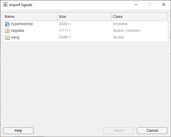
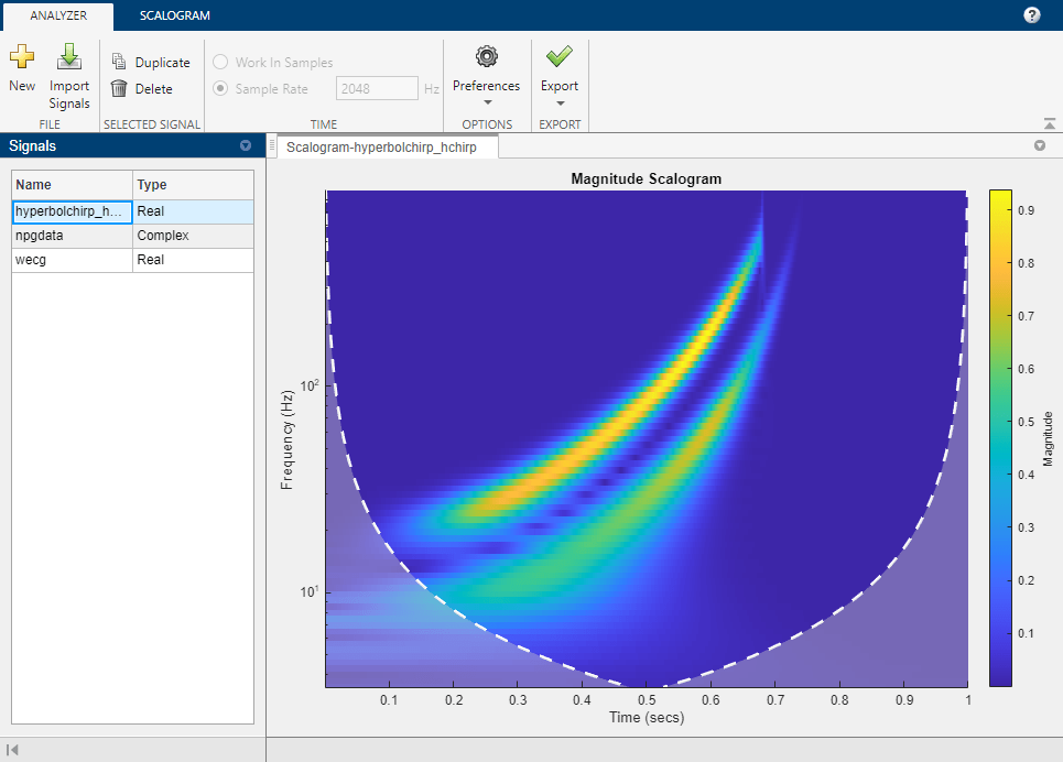
Select all the signals and click Import. After a brief, one-time initialization, the Signals pane is populated with the names of the imported signals, along with their types. In the case of hyperbolchirp, the name of the timetable variable containing the signal is appended to the name of the timetable: hyperbolchirp_hchirp. The app displays the scalogram of the highlighted signal. The scalogram is obtained using the cwt function with default settings. The cone of influence showing where edge effects become significant is also plotted. Gray regions outside the dashed white lines delineate regions where edge effects are significant. By default, frequencies are in cycles/sample.
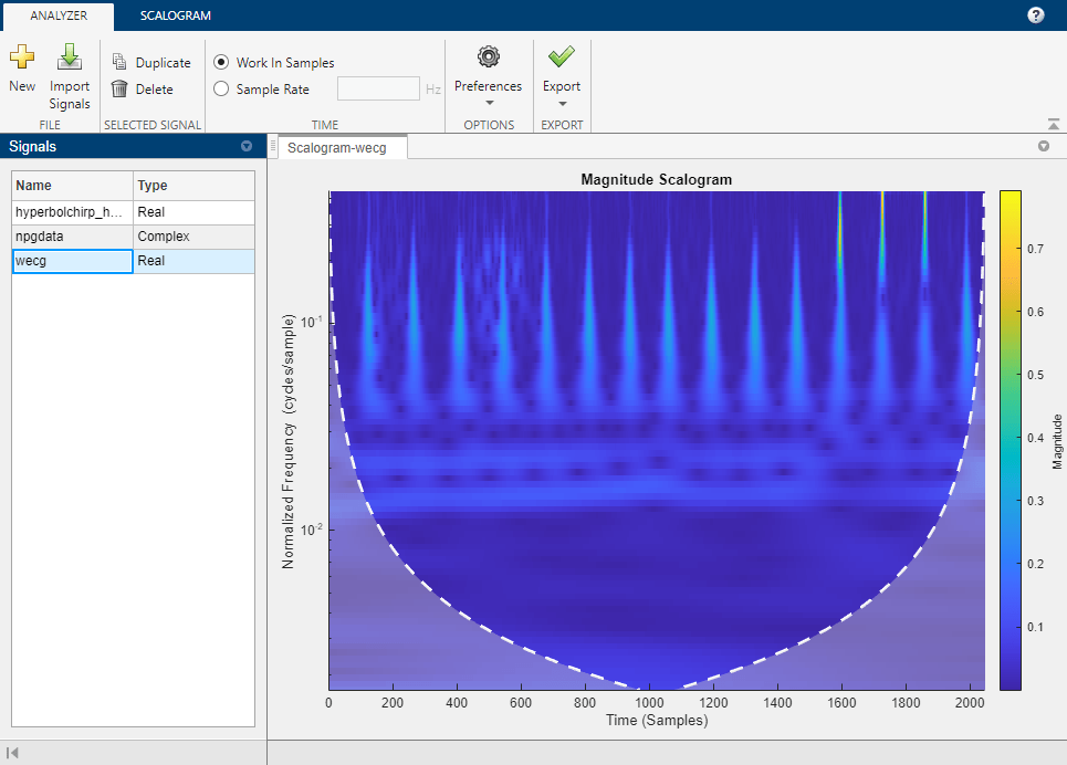
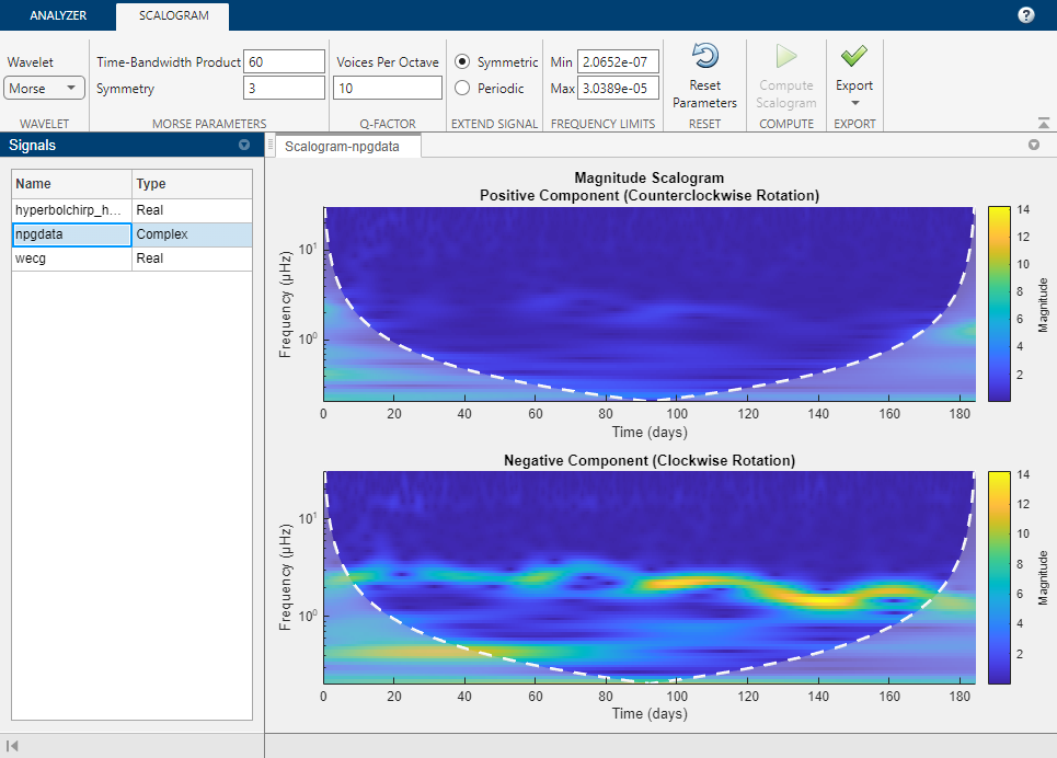
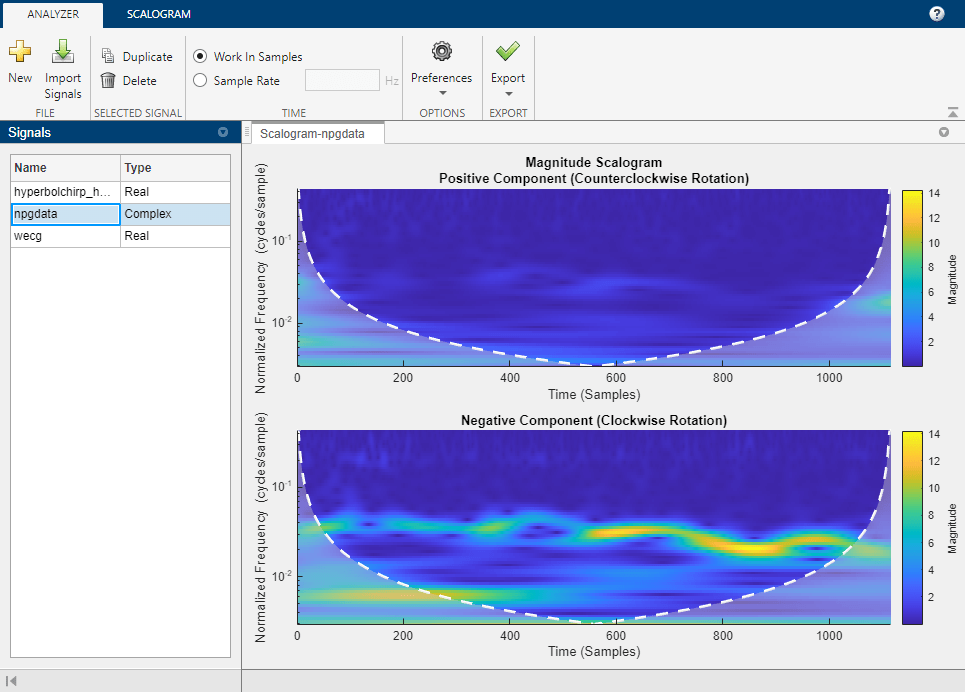
The ECG signal is real valued. In the Signals pane, select the complex-valued signal npgdata. The positive and negative components of the scalogram are displayed.
Select hyperbolchirp_hchirp. Because the timetable contains temporal information, the scalogram is plotted as a function of frequency in hertz and uses the row times of the timetable as the basis for the time axis. The disabled Sample Rate field displays the sampling rate as determined from the row times.
Load the hyperbolic chirp signal.
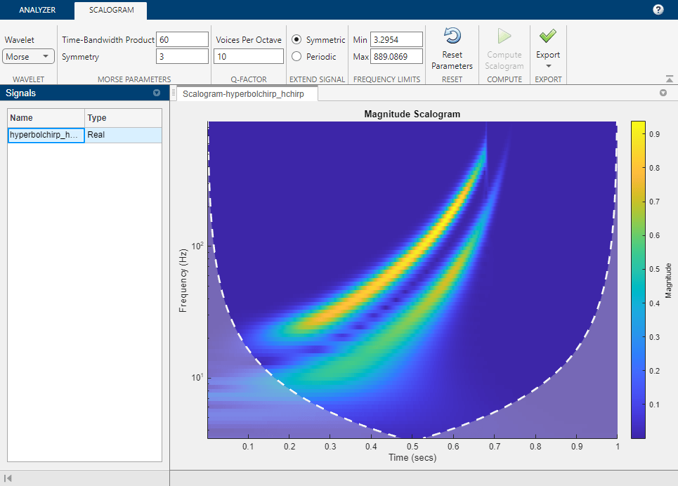
load hyperbolchirpOpen Wavelet Time-Frequency Analyzer and import the signal into the app. To access the parameter settings, click the Scalogram tab. By default, the app displays the scalogram obtained using the analytic Morse (3, 60) wavelet and the cwt function with default settings.
You can reset the CWT parameters to their default values at any time by clicking Reset Parameters. Resetting the parameters enables the Compute Scalogram button.
To visualize the scalogram using the (1,5) Morse wavelet, set Time-Bandwidth Product to 5. In the status bar, text appears stating there are pending changes. The Compute Scalogram button is now enabled. If you instead first set Symmetry to 1, the app would automatically change that value because a symmetry value of 1 violates the constraint that the ratio of Time-Bandwidth Product to Symmetry should not exceed 40. For more information, see Tips.
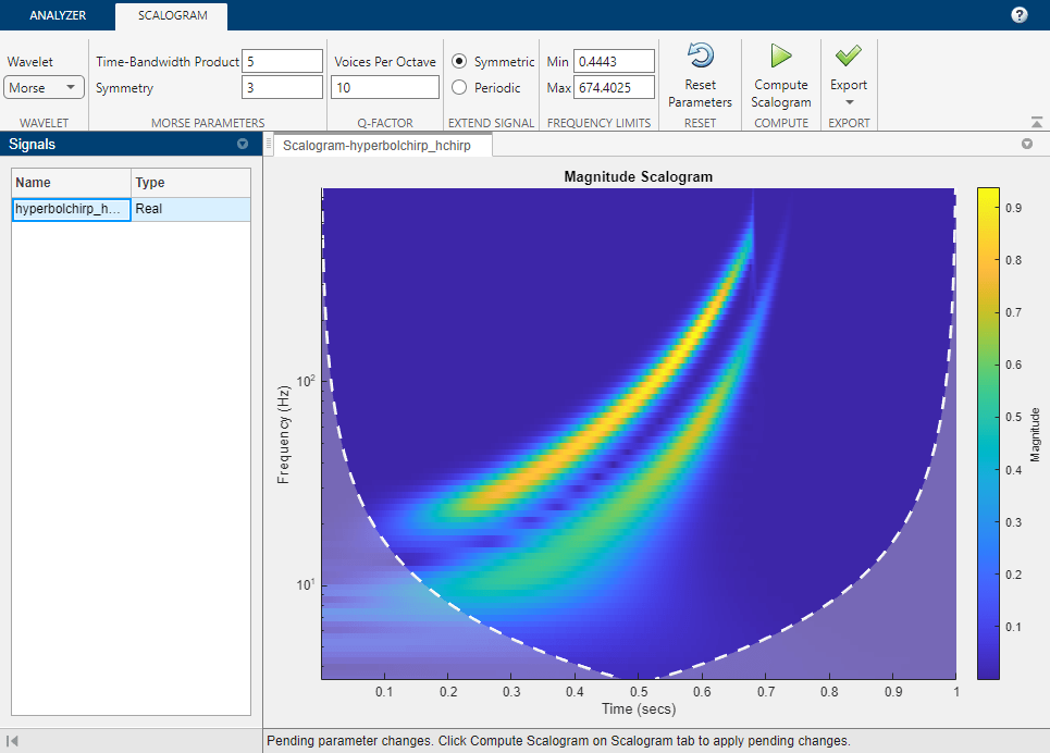
Now set Symmetry to 1 and click Compute Scalogram. The app displays the scalogram obtained using the (1, 5) Morse wavelet.

To visualize the scalogram using the (6, 50) Morse wavelet, first set Time-Bandwidth Product to 50 and Symmetry to 6, then click Compute Scalogram.
Since R2026a
Import Signal
Load a hyperbolic chirp signal into your workspace.
load hyperbolchirpVisualize Scalogram
Open Wavelet Time-Frequency Analyzer and import the signal. To access the parameter settings, click the Scalogram tab. By default, the app displays the scalogram obtained using the Morse (3,60) wavelet and the cwt function with default settings. Because the signal is a timetable, the scalogram is plotted as a function of frequency in hertz. The time axis is based on the row times of the timetable.
In the Scalogram tab, adjust the default settings. Specify the Morse (5,20) wavelet. Visualize the scalogram using 26 voices per octave and zero padding boundary extension. The frequencies are plotted on a logarithmic scale.

Generate Script
To adjust the frequency axis scale in the scalogram, first reproduce the wavelet analysis in your workspace.
Generate a script that recreates the scalogram in your workspace. From the Export ▼ menu, select Generate MATLAB Script. An untitled script opens in your MATLAB® Editor. To include the boundary line of the cone of influence in the plot, add a third output argument, coi, to the cwt function call in the script. Save and execute the script. The variables scalogram and frequency contain the scalogram and frequency vector, respectively.
%Parameters
waveletParameters = [5,20];
voicesPerOctave = 26;
boundary = "zeropad";
%Compute CWT
%If necessary, substitute workspace variable name for hyperbolchirp as first input to cwt() function in code below
%Run the function call below without output arguments to plot the results
[waveletTransform,frequency,coi] = cwt(hyperbolchirp,...
    WaveletParameters=waveletParameters,...
    VoicesPerOctave=voicesPerOctave,...
    Boundary=boundary);
scalogram = abs(waveletTransform);
In order to plot the scalogram using the correct time axis, extract the vector of row times, Time, from the hyperbolchirp timetable.
dataTimes = hyperbolchirp.Time;
Adjust Frequency Axis — Linear Scale
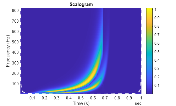
Use the pcolor function to plot the scalogram. Include the cone of influence boundary. Frequency is plotted on a linear scale.
pcolor(dataTimes,frequency,scalogram)
shading flat
title("Scalogram")
xlabel("Time (s)")
ylabel("Frequency (Hz)")
hold on
plot(dataTimes,coi,"w--",LineWidth=2)
hold off
colorbar
Adjust Frequency Axis — Logarithmic Scale
To plot frequency on a logarithmic scale, get the handle to the current axes and set YScale to "log".
AX = gca;
set(AX,YScale="log")
In MATLAB, logarithmic axes are in powers of 10 (decades). By default, MATLAB places frequency ticks at 1, 10, and 100 because they are the powers of 10 between the minimum and maximum frequencies. To add more frequency axis ticks, obtain the minimum and maximum frequencies in frequency. Create a logarithmically spaced set of frequencies between the minimum and maximum frequencies. Note that cwt returns frequencies ordered from high to low.
minf = frequency(end);
maxf = frequency(1);
numfreq = 10;
freq = logspace(log10(minf),log10(maxf),numfreq);
Replace the frequency axis ticks and labels with the new frequencies.
AX.YTickLabelMode = "auto";
AX.YTick = freq;
In the CWT, frequencies are computed in powers of two. Create the frequency ticks and tick labels in powers of two.
freq = 2.^(round(log2(minf)):round(log2(maxf)));
AX.YTickLabelMode = "auto";
AX.YTick = freq;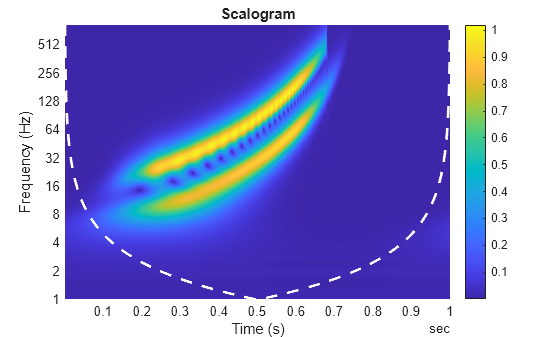
Related Examples
Parameters
Programmatic Use
Limitations
The MATLAB script you generate to create the scalogram in your workspace uses the name of the selected signal in the Signals pane. The script will throw an error if the variable does not exist in the MATLAB workspace. If an error occurs, either replace the variable name in the script with the name of the original signal or create the variable in your workspace.
Tips
The Morse wavelet parameters, Time-Bandwidth Product and Symmetry, must satisfy three constraints:
Symmetry, or gamma, must be greater than or equal to 1.
Time-Bandwidth Product must be greater than or equal to Symmetry.
The ratio of Time-Bandwidth Product to Symmetry cannot exceed 40.
To prevent attempts to visualize a scalogram using invalid settings, the app validates any parameter you change. If you enter a value that violates a constraint, the app automatically replaces it with a valid value. The new value might not be the desired value. To avoid unexpected results, you should ensure any value you enter always results in a valid setting. For more information, see the example Adjust Morse Wavelet Parameters.
Version History
Introduced in R2022aSee Also
Apps
- Wavelet Signal Analyzer | Signal Multiresolution Analyzer | Signal Analyzer (Signal Processing Toolbox)