Train Classification Network to Classify Object in 3-D Point Cloud

This example uses:

This example demonstrates the approach outlined in [1] in which point cloud data is preprocessed into a voxelized encoding and then used directly with a simple 3-D convolutional neural network (CNN) architecture to perform object classification. In more recent approaches such as [2], encodings of point cloud data can be more complicated and can be learned encodings that are trained end-to-end along with a network performing a classification/object detection/segmentation task. However, the general pattern of moving from irregular unordered points to a gridded structure that can be fed into CNNs remains similar in all of these approaches.

Import and Analyze Data

In this example, we work with the Sydney Urban Objects Dataset. In this example, use folds 1-3 from the data as the training set and fold 4 as the validation set.

dataPath = downloadSydneyUrbanObjects(tempdir);
dsTrain = loadSydneyUrbanObjectsData(dataPath,[1 2 3]);
dsVal = loadSydneyUrbanObjectsData(dataPath,4);

Analyze the training set to understand the labels present in the data and the overall distribution of labels.

dsLabels = transform(dsTrain,@(data) data{2});
labels = readall(dsLabels);
figure
histogram(labels)

From the histogram, it is apparent that there is a class imbalance issue in the training data in which certain object classes like Car and Pedestrian are much more common than less frequent classes like Ute.

Data Augmentation

To avoid overfitting and add robustness to a classifier, some amount of randomized data augmentation is generally a good idea when training a network. The functions randomAffine2d and pctransform make it easy to define randomized affine transformations on point cloud data. We additionally add some randomized per-point jitter to each point in every point cloud. The function augmentPointCloudData is included in the supporting functions section below.

dsTrain = transform(dsTrain,@augmentPointCloudData);

Verify that augmentation of point cloud data looks reasonable.

dataOut = preview(dsTrain);
figure
pcshow(dataOut{1});
title(dataOut{2});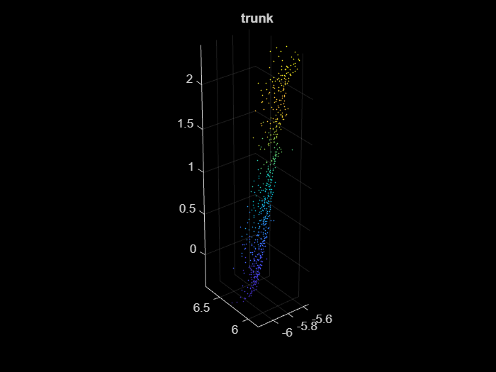

We next add a simple voxelization transform to each input point cloud as discussed in the previous example, to transform our input point cloud into a pseudo-image that can be used with a CNN. Use a simple occupancy grid.

dsTrain = transform(dsTrain,@formOccupancyGrid);
dsVal = transform(dsVal,@formOccupancyGrid);

Examine a sample of the final voxelized volume that we will feed into the network to verify that voxelization is working correctly.

data = preview(dsTrain);
figure
p = patch(isosurface(data{1},0.5));
p.FaceColor = "red";
p.EdgeColor = "none";
daspect([1 1 1])
view(45,45)
camlight; 
lighting phong
title(data{2});

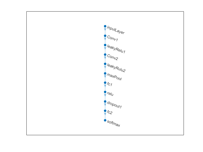
Define Network Architecture

In this example, we use a simple 3-D classification architecture as described in [1].

layers = [image3dInputLayer([32 32 32],Name="inputLayer",Normalization="none"),...
    convolution3dLayer(5,32,Stride=2,Name="Conv1"),...
    leakyReluLayer(0.1,Name="leakyRelu1"),...
    convolution3dLayer(3,32,Stride=1,Name="Conv2"),...
    leakyReluLayer(0.1,Name="leakyRulu2"),...
    maxPooling3dLayer(2,Stride=2,Name="maxPool"),...
    fullyConnectedLayer(128,Name="fc1"),...
    reluLayer(Name="relu"),...
    dropoutLayer(0.5,Name="dropout1"),...
    fullyConnectedLayer(14,Name="fc2"),...
    softmaxLayer(Name="softmax")];

voxnet = dlnetwork(layers);
figure
plot(voxnet);

Setup Training Options

Use stochastic gradient descent with momentum with a piecewise adjustment to the learning rate schedule. This example was run on a TitanX GPU. If your GPU has less memory, it may be necessary to reduce the batch size. Though 3-D CNNs have an advantage of conceptual simplicity, they have the drawback of large amounts of memory usage at training time.

miniBatchSize = 32;
dsLength = length(dsTrain.UnderlyingDatastore.Files);
iterationsPerEpoch = floor(dsLength/miniBatchSize);
dropPeriod = floor(8000/iterationsPerEpoch);

options = trainingOptions("sgdm",...
    InitialLearnRate=0.01,...
    MiniBatchSize=miniBatchSize,...
    LearnRateSchedule="Piecewise",...
    LearnRateDropPeriod=dropPeriod,...
    ValidationData=dsVal, ...
    MaxEpochs=60,...
    DispatchInBackground=false,...
    Shuffle="never");

Train Network

Train the neural network using the trainnet (Deep Learning Toolbox) function. For classification, use cross-entropy loss.

voxnet = trainnet(dsTrain,voxnet,"crossentropy",options);

    Iteration    Epoch    TimeElapsed    LearnRate    TrainingLoss    ValidationLoss
    _________    _____    ___________    _________    ____________    ______________
            0        0       00:00:07         0.01                             2.649
            1        1       00:00:08         0.01          2.6395                  
           50        4       00:00:30         0.01          2.0839            2.3076
          100        8       00:00:53         0.01          2.3592            2.2487
          150       12       00:01:16         0.01          2.2527            1.9915
          200       16       00:01:38         0.01          2.0546            1.8198
          250       20       00:02:01         0.01          1.6182            1.5325
          300       24       00:02:23         0.01          1.7817            1.4501
          350       27       00:02:45         0.01          1.5115            1.2817
          400       31       00:03:07         0.01          1.2351            1.2655
          450       35       00:03:30         0.01          1.5587            1.2746
          500       39       00:03:52         0.01          1.3871            1.3286
          550       43       00:04:17         0.01          1.4678            1.1589
          600       47       00:04:39         0.01          1.4869             1.175
          650       50       00:05:01         0.01         0.92234            1.1875
          700       54       00:05:23         0.01         0.90772            1.1278
          750       58       00:05:45         0.01          1.1843            1.1523
          780       60       00:05:58         0.01         0.90802            1.0837
Training stopped: Max epochs completed

Evaluate Network

Following the structure of [1], this example only forms a training and validation set from Sydney Urban Objects. Evaluate the performance of the trained network using the validation, since it was not used to train the network.

valLabelSet = transform(dsVal,@(data) data{2});
valLabels = readall(valLabelSet);
outputScores = minibatchpredict(voxnet,dsVal);
outputLabels = scores2label(outputScores,categories(labels));
accuracy = nnz(outputLabels == valLabels) / numel(outputLabels);
disp(accuracy)

    0.6903

View the confusion matrix to study the accuracy across the various label categories.

confusionchart(valLabels,outputLabels)

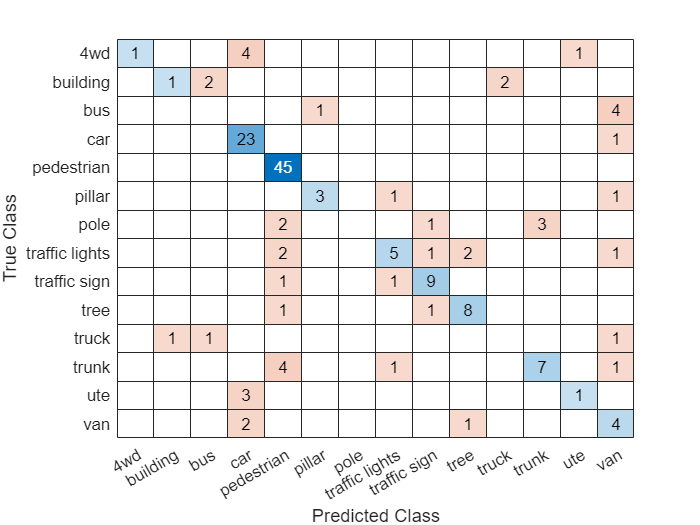
The label imbalance noted in the training set is an issue in the classification accuracy. The confusion chart illustrates higher precision and recall for pedestrian, the most common class, than for less common classes like van. Since the purpose of this example is to demonstrate a basic classification network training approach with point cloud data, possible next steps that could be taken to improve classification performance such as resampling the training set or achieve better label balance or using a loss function more robust to label imbalance (e.g. weighted cross-entropy) will not be explored.

Supporting Functions

function datasetPath = downloadSydneyUrbanObjects(dataLoc)

if nargin == 0
    dataLoc = pwd();
end

dataLoc = string(dataLoc);

url = "http://www.acfr.usyd.edu.au/papers/data/";
name = "sydney-urban-objects-dataset.tar.gz";

if ~exist(fullfile(dataLoc,"sydney-urban-objects-dataset"),"dir")
    disp("Downloading Sydney Urban Objects Dataset...");
    untar(url+name,dataLoc);
end

datasetPath = fullfile(dataLoc,"sydney-urban-objects-dataset");

end

function ds = loadSydneyUrbanObjectsData(datapath,folds)
% loadSydneyUrbanObjectsData Datastore with point clouds and
% associated categorical labels for Sydney Urban Objects dataset.
%
% ds = loadSydneyUrbanObjectsData(datapath) constructs a datastore that
% represents point clouds and associated categories for the Sydney Urban
% Objects dataset. The input, datapath, is a string or char array which
% represents the path to the root directory of the Sydney Urban Objects
% Dataset.
%
% ds = loadSydneyUrbanObjectsData(___,folds) optionally allows
% specification of desired folds that you wish to be included in the
% output ds. For example, [1 2 4] specifies that you want the first,
% second, and fourth folds of the Dataset. Default: [1 2 3 4].

if nargin < 2
    folds = 1:4;
end

datapath = string(datapath);
path = fullfile(datapath,"objects",filesep);

% For now, include all folds in Datastore
foldNames{1} = importdata(fullfile(datapath,'folds','fold0.txt'));
foldNames{2} = importdata(fullfile(datapath,'folds','fold1.txt'));
foldNames{3} = importdata(fullfile(datapath,'folds','fold2.txt'));
foldNames{4} = importdata(fullfile(datapath,'folds','fold3.txt'));
names = foldNames(folds);
names = vertcat(names{:});

fullFilenames = append(path,names);
ds = fileDatastore(fullFilenames,ReadFcn=@extractTrainingData,FileExtensions=".bin");

% Shuffle
ds.Files = ds.Files(randperm(length(ds.Files)));

end

function dataOut = extractTrainingData(fname)

[pointData,intensity] = readbin(fname);

[~,name] = fileparts(fname);
name = string(name);
name = extractBefore(name,'.');
name = replace(name,'_',' ');

labelNames = ["4wd","building","bus","car","pedestrian","pillar",...
    "pole","traffic lights","traffic sign","tree","truck","trunk","ute","van"];

label = categorical(name,labelNames);

dataOut = {pointCloud(pointData,'Intensity',intensity),label};

end

function [pointData,intensity] = readbin(fname)
% readbin Read point and intensity data from Sydney Urban Object binary
% files.

% names = ['t','intensity','id',...
%          'x','y','z',...
%          'azimuth','range','pid']
% 
% formats = ['int64', 'uint8', 'uint8',...
%            'float32', 'float32', 'float32',...
%            'float32', 'float32', 'int32']

fid = fopen(fname, 'r');
c = onCleanup(@() fclose(fid));
    
fseek(fid,10,-1); % Move to the first X point location 10 bytes from beginning
X = fread(fid,inf,'single',30);
fseek(fid,14,-1);
Y = fread(fid,inf,'single',30);
fseek(fid,18,-1);
Z = fread(fid,inf,'single',30);

fseek(fid,8,-1);
intensity = fread(fid,inf,'uint8',33);

pointData = [X,Y,Z];

end

function dataOut = formOccupancyGrid(data)

grid = pcbin(data{1},[32 32 32]);
occupancyGrid = zeros(size(grid),'single');
for ii = 1:numel(grid)
    occupancyGrid(ii) = ~isempty(grid{ii});
end
label = data{2};
dataOut = {occupancyGrid,label};

end

function dataOut = augmentPointCloudData(data)

ptCloud = data{1};
label = data{2};

% Apply randomized rotation about Z axis.
tform = randomAffine3d(Rotation=@() deal([0 0 1],360*rand),Scale=[0.98,1.02], ...
   XReflection=true,YReflection=true); % Randomized rotation about z axis
ptCloud = pctransform(ptCloud,tform);

% Apply jitter to each point in point cloud
amountOfJitter = 0.01;
numPoints = size(ptCloud.Location,1);
D = zeros(size(ptCloud.Location),'like',ptCloud.Location);
D(:,1) = diff(ptCloud.XLimits)*rand(numPoints,1);
D(:,2) = diff(ptCloud.YLimits)*rand(numPoints,1);
D(:,3) = diff(ptCloud.ZLimits)*rand(numPoints,1);
D = amountOfJitter.*D;
ptCloud = pctransform(ptCloud,D);

dataOut = {ptCloud,label};

end

References

1) Voxnet: A 3d convolutional neural network for real-time object recognition, Daniel Maturana, Sebastian Scherer, 2015 IEEE/RSJ International Conference on Intelligent Robots and Systems (IROS).

2) PointPillars: Fast Encoders for Object Detection from Point Clouds, Alex H. Lang, Sourabh Vora, et al, CVPR 2019.

3) Sydney Urban Objects Dataset, Alastair Quadros, James Underwood, Bertrand Douillard, Sydney Urban Objects.

How useful was this information?

Unrated 1 star 2 stars 3 stars 4 stars 5 stars