Object Detection Using Custom Training Loop

This example shows how to train a YOLO v3 object detector using custom training loop.

Deep learning is a powerful machine learning technique that you can use to train robust object detectors. Several techniques for object detection exist, including Faster R-CNN, you only look once (YOLO) v2, and single shot detector (SSD). YOLO v3 improves upon YOLO v2 by adding detection at multiple scales to help detect smaller objects. This example shows how to train a YOLO v3 object detector using a custom training loop. The loss function used for training the YOLO v3 object detector is separated into mean squared error for bounding box regression and binary cross-entropy for object classification to help improve detection accuracy. Training using custom training loops provides several benefits which include flexibility to define custom metrics and custom loss functions. It also provides the ability to train complex deep learning architectures with complete control over training process.

Download Pretrained Network

Download a pretrained network by using the helper function downloadPretrainedYOLOv3Detector to avoid having to wait for training to complete. If you want to train the network with a new set of data, set the doTraining variable to true.

doTraining = false;

if ~doTraining
    preTrainedDetector = downloadPretrainedYOLOv3Detector();    
end

Downloading pretrained detector...

Load Data

This example uses a small labeled data set that contains 295 images. Many of these images come from the Caltech Cars 1999 and 2001 data sets, created by Pietro Perona and used with permission. Each image contains one or two labeled instances of a vehicle. A small data set is useful for exploring the YOLO v3 training procedure, but in practice, more labeled images are needed to train a robust network.

Unzip the vehicle images and load the vehicle ground truth data.

unzip vehicleDatasetImages.zip
data = load('vehicleDatasetGroundTruth.mat');
vehicleDataset = data.vehicleDataset;

% Add the full path to the local vehicle data folder.
vehicleDataset.imageFilename = fullfile(pwd, vehicleDataset.imageFilename);

Note: In case of multiple classes, the data can also be organized as three columns where the first column contains the image file names with paths, the second column contains the bounding boxes and the third column must be a cell vector that contains the label names corresponding to each bounding box. For more information on how to arrange the bounding boxes and labels, see boxLabelDatastore.

All the bounding boxes must be in the form [x y width height]. This vector specifies the upper left corner and the size of the bounding box in pixels.

Split the data set into a training set for training the network, and a test set for evaluating the network. Use 60% of the data for training set and the rest for the test set.

rng(0);
shuffledIndices = randperm(height(vehicleDataset));
idx = floor(0.6 * length(shuffledIndices));
trainingDataTbl = vehicleDataset(shuffledIndices(1:idx), :);
testDataTbl = vehicleDataset(shuffledIndices(idx+1:end), :);

Create an image datastore for loading the images.

imdsTrain = imageDatastore(trainingDataTbl.imageFilename);
imdsTest = imageDatastore(testDataTbl.imageFilename);

Create a datastore for the ground truth bounding boxes.

bldsTrain = boxLabelDatastore(trainingDataTbl(:, 2:end));
bldsTest = boxLabelDatastore(testDataTbl(:, 2:end));

Combine the image and box label datastores.

trainingData = combine(imdsTrain, bldsTrain);
testData = combine(imdsTest, bldsTest);

Use validateInputData to detect invalid images, bounding boxes or labels i.e.,

• Samples with invalid image format or containing NaNs

• Bounding boxes containing zeros/NaNs/Infs/empty

• Missing/non-categorical labels.

The values of the bounding boxes should be finite, positive, non-fractional, non-NaN and should be within the image boundary with a positive height and width. Any invalid samples must either be discarded or fixed for proper training.

validateInputData(trainingData);
validateInputData(testData);

Data Augmentation

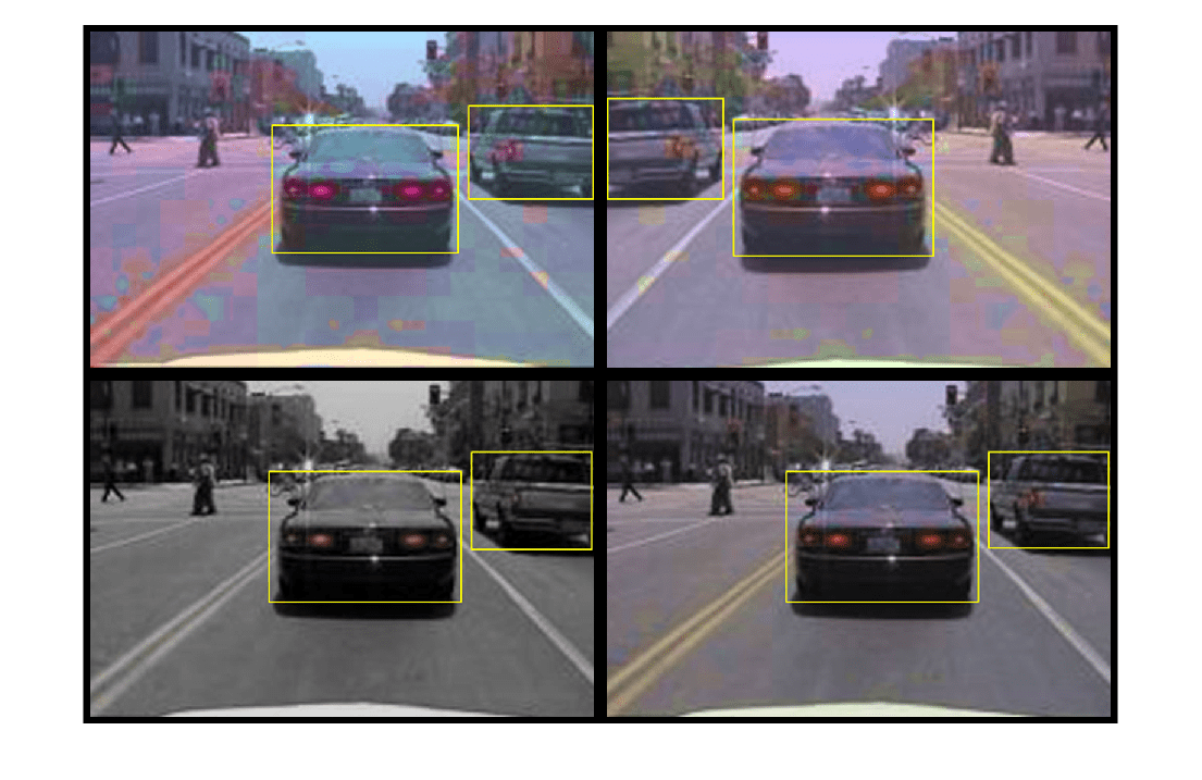
Data augmentation is used to improve network accuracy by randomly transforming the original data during training. By using data augmentation, you can add more variety to the training data without actually having to increase the number of labeled training samples.

Use transform function to apply custom data augmentations to the training data. The augmentData helper function, listed at the end of the example, applies the following augmentations to the input data.

• Color jitter augmentation in HSV space

• Random horizontal flip

• Random scaling by 10 percent

augmentedTrainingData = transform(trainingData, @augmentData);

Read the same image four times and display the augmented training data.

augmentedData = cell(4,1);
for k = 1:4
    data = read(augmentedTrainingData);
    augmentedData{k} = insertShape(data{1,1},"Rectangle",data{1,2});
    reset(augmentedTrainingData);
end
figure
montage(augmentedData,BorderSize=10)

Define YOLO v3 Object Detector

The YOLO v3 detector in this example is based on SqueezeNet, and uses the feature extraction network in SqueezeNet with the addition of two detection heads at the end. The second detection head is twice the size of the first detection head, so it is better able to detect small objects. Note that you can specify any number of detection heads of different sizes based on the size of the objects that you want to detect. The YOLO v3 detector uses anchor boxes estimated using training data to have better initial priors corresponding to the type of data set and to help the detector learn to predict the boxes accurately. For information about anchor boxes, see Anchor Boxes for Object Detection.

The YOLO v3 network present in the YOLO v3 detector is illustrated in the following diagram.

You can use Deep Network Designer (Deep Learning Toolbox) to create the network shown in the diagram.

Specify the network input size. When choosing the network input size, consider the minimum size required to run the network itself, the size of the training images, and the computational cost incurred by processing data at the selected size. When feasible, choose a network input size that is close to the size of the training image and larger than the input size required for the network. To reduce the computational cost of running the example, specify a network input size of [227 227 3].

networkInputSize = [227 227 3];

First, use transform to preprocess the training data for computing the anchor boxes, as the training images used in this example are bigger than 227-by-227 and vary in size. Specify the number of anchors as 6 to achieve a good tradeoff between number of anchors and mean IoU. Use the estimateAnchorBoxes function to estimate the anchor boxes. For details on estimating anchor boxes, see Estimate Anchor Boxes From Training Data. In case of using a pretrained YOLOv3 object detector, the anchor boxes calculated on that particular training dataset need to be specified. Note that the estimation process is not deterministic. To prevent the estimated anchor boxes from changing while tuning other hyperparameters, set the random seed prior to estimation using rng.

rng(0)
trainingDataForEstimation = transform(trainingData, @(data)preprocessData(data, networkInputSize));
numAnchors = 6;
[anchors, meanIoU] = estimateAnchorBoxes(trainingDataForEstimation, numAnchors)

anchors = 6×2

    42    37
   160   130
    96    92
   141   123
    35    25
    69    66

meanIoU = 0.8430

Specify anchorBoxes to use in both the detection heads. anchorBoxes is a cell array of [Mx1], where M denotes the number of detection heads. Each detection head consists of a [Nx2] matrix of anchors, where N is the number of anchors to use. Select anchorBoxes for each detection head based on the feature map size. Use larger anchors at lower scale and smaller anchors at higher scale. To do so, sort the anchors with the larger anchor boxes first and assign the first three to the first detection head and the next three to the second detection head.

area = anchors(:, 1).*anchors(:, 2);
[~, idx] = sort(area,"descend");
anchors = anchors(idx, :);
anchorBoxes = {anchors(1:3,:)
    anchors(4:6,:)
    };

Load the SqueezeNet network pretrained on Imagenet data set and then specify the class names. You can also choose to load a different pretrained network trained on COCO data set such as tiny-yolov3-coco or darknet53-coco or Imagenet data set such as MobileNet-v2 or ResNet-18. YOLO v3 performs better and trains faster when you use a pretrained network.

baseNetwork = imagePretrainedNetwork("squeezenet");
classNames = trainingDataTbl.Properties.VariableNames(2:end);

Next, create the yolov3ObjectDetector object by adding the detection network source. Choosing the optimal detection network source requires trial and error, and you can use analyzeNetwork to find the names of potential detection network source within a network. For this example, use the fire9-concat and fire5-concat layers as DetectionNetworkSource.

yolov3Detector = yolov3ObjectDetector(baseNetwork,classNames,anchorBoxes, ...
    DetectionNetworkSource=["fire9-concat","fire5-concat"],InputSize=networkInputSize);

Alternatively, instead of the network created above using SqueezeNet, other pretrained YOLOv3 architectures trained using larger datasets like MS-COCO can be used to transfer learn the detector on custom object detection task. Transfer learning can be realized by changing the classNames and anchorBoxes.

Preprocess Training Data

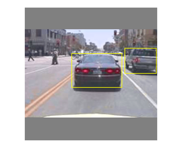
Preprocess the augmented training data to prepare for training. The preprocess method in yolov3ObjectDetector, applies the following preprocessing operations to the input data.

• Resize the images to the network input size by maintaining the aspect ratio.

• Scale the image pixels in the range [0 1].

preprocessedTrainingData = transform(augmentedTrainingData, @(data)preprocess(yolov3Detector,data));

Read the preprocessed training data.

data = read(preprocessedTrainingData);

Display the image with the bounding boxes.

I = data{1,1};
bbox = data{1,2};
annotatedImage = insertShape(I, "Rectangle", bbox);
annotatedImage = imresize(annotatedImage,2);
figure
imshow(annotatedImage)

Reset the datastore.

reset(preprocessedTrainingData);

Specify Training Options

Specify these training options.

• Set the number of epochs to be 80.

• Set the mini batch size as 8. Stable training can be possible with higher learning rates when higher mini batch size is used. Although, this should be set depending on the available memory.

• Set the learning rate to 0.001.

• Set the warmup period as 1000 iterations. This parameter denotes the number of iterations to increase the learning rate exponentially based on the formula $$\text{learningRate}\times {\left(\frac{\text{iteration}}{\text{warmupPeriod}}\right)}^4$$. It helps in stabilizing the gradients at higher learning rates.

• Set the L2 regularization factor to 0.0005.

• Specify the penalty threshold as 0.5. Detections that overlap less than 0.5 with the ground truth are penalized.

• Initialize the velocity of gradient as []. This is used by SGDM to store the velocity of gradients.

numEpochs = 80;
miniBatchSize = 8;
learningRate = 0.001;
warmupPeriod = 1000;
l2Regularization = 0.0005;
penaltyThreshold = 0.5;
velocity = [];

Train Model

This example demonstrates training YOLO v3 object detector using custom training loop. Train on a GPU, if one is available. Using a GPU requires Parallel Computing Toolbox™ and a CUDA® enabled NVIDIA® GPU. For information about the supported compute capabilities, see GPU Computing Requirements (Parallel Computing Toolbox).

Use the minibatchqueue function to split the preprocessed training data into batches with the supporting function createBatchData which returns the batched images and bounding boxes combined with the respective class IDs. For faster extraction of the batch data for training, dispatchInBackground should be set to "true" which ensures the usage of parallel pool.

minibatchqueue automatically detects the availability of a GPU. If you do not have a GPU, or do not want to use one for training, set the OutputEnvironment parameter to "cpu".

if canUseParallelPool
   dispatchInBackground = true;
else
   dispatchInBackground = false;
end

mbqTrain = minibatchqueue(preprocessedTrainingData,2,...
        MiniBatchSize=miniBatchSize,...
        MiniBatchFcn=@(images,boxes,labels) createBatchData(images,boxes,labels,classNames), ...
        MiniBatchFormat=["SSCB", ""],...
        DispatchInBackground=dispatchInBackground,...
        OutputCast=["", "double"]);

Create the training progress plotter using supporting function configureTrainingProgressPlotter to see the plot while training the detector object with a custom training loop.

Finally, specify the custom training loop. For each iteration:

• Read data from the minibatchqueue. If it does not have any more data, reset the minibatchqueue and shuffle.

• Evaluate the model gradients using dlfeval and the modelGradients function. The function modelGradients, listed as a supporting function, returns the gradients of the loss with respect to the learnable parameters in net, the corresponding mini-batch loss, and the state of the current batch.

• Apply a weight decay factor to the gradients to regularization for more robust training.

• Determine the learning rate based on the iterations using the piecewiseLearningRateWithWarmup supporting function.

• Update the detector parameters using the sgdmupdate function.

• Update the state parameters of detector with the moving average.

• Display the learning rate, total loss, and the individual losses (box loss, object loss and class loss) for every iteration. These can be used to interpret how the respective losses are changing in each iteration. For example, a sudden spike in the box loss after few iterations implies that there are Inf or NaNs in the predictions.

• Update the training progress plot.

The training can also be terminated if the loss has saturated for few epochs.

if doTraining
    
    % Create subplots for the learning rate and mini-batch loss.
    fig = figure;
    [lossPlotter, learningRatePlotter] = configureTrainingProgressPlotter(fig);

    iteration = 0;
    % Custom training loop.
    for epoch = 1:numEpochs
          
        reset(mbqTrain);
        shuffle(mbqTrain);
        
        while(hasdata(mbqTrain))
            iteration = iteration + 1;
           
            [XTrain, YTrain] = next(mbqTrain);
            
            % Evaluate the model gradients and loss using dlfeval and the
            % modelGradients function.
            [gradients, state, lossInfo] = dlfeval(@modelGradients, yolov3Detector, XTrain, YTrain, penaltyThreshold);
    
            % Apply L2 regularization.
            gradients = dlupdate(@(g,w) g + l2Regularization*w, gradients, yolov3Detector.Learnables);
    
            % Determine the current learning rate value.
            currentLR = piecewiseLearningRateWithWarmup(iteration, epoch, learningRate, warmupPeriod, numEpochs);
    
            % Update the detector learnable parameters using the SGDM optimizer.
            [yolov3Detector.Learnables, velocity] = sgdmupdate(yolov3Detector.Learnables, gradients, velocity, currentLR);
    
            % Update the state parameters of dlnetwork.
            yolov3Detector.State = state;
              
            % Display progress.
            displayLossInfo(epoch, iteration, currentLR, lossInfo);  
                
            % Update training plot with new points.
            updatePlots(lossPlotter, learningRatePlotter, iteration, currentLR, lossInfo.totalLoss);
        end        
    end
else
    yolov3Detector = preTrainedDetector;
end

Evaluate Model

Run the detector on all the test images. Set the detection threshold to a low value to detect as many objects as possible. This helps you evaluate the detector precision across the full range of recall values.

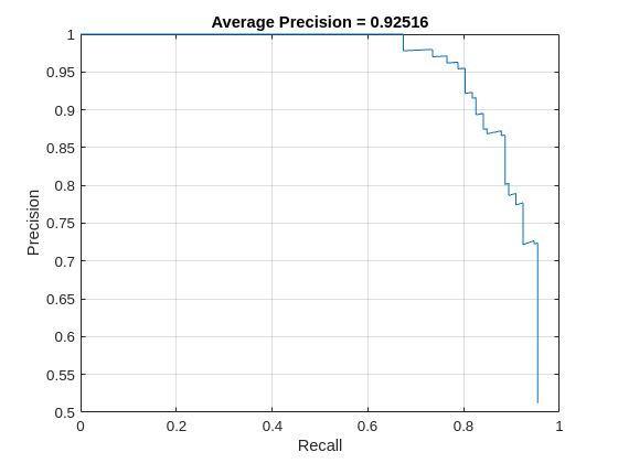
Measure the average precision using the evaluateObjectDetection function. The average precision provides a single number that incorporates the ability of the detector to make correct classifications (precision) and the ability of the detector to find all relevant objects (recall).

results = detect(yolov3Detector,testData,MiniBatchSize=8,Threshold=0.01);

% Evaluate the object detector using Average Precision metric.
classID = 1;
metrics = evaluateObjectDetection(results,testData);
[precision,recall] = precisionRecall(metrics,ClassName="vehicle");

The precision-recall (PR) curve shows how precise a detector is at varying levels of recall. Ideally, the precision is 1 at all recall levels. Plot the PR curve.

figure
plot(recall{:},precision{:})
xlabel("Recall")
ylabel("Precision")
grid on
title("Average Precision = "+averagePrecision(metrics,ClassName="vehicle"))

Detect Objects Using YOLO v3

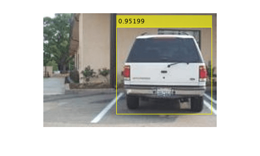
Use the detector for object detection.

% Read the datastore.
data = read(testData);

% Get the image.
I = data{1};

[bboxes,scores,labels] = detect(yolov3Detector,I);

% Display the detections on image.
I = insertObjectAnnotation(I,"rectangle",bboxes,scores);

figure
imshow(I)

Further Exploration

• To can train a YOLO v3 object detection network using the trainYOLOv3ObjectDetector function, see Object Detection Using YOLO v3 Deep Learning example. This function mitigates the need to write a custom training loop and supports advanced operations such as parallel and multi-GPU training.

• You can increase the training speed and reduce memory consumption by freezing the subnetworks of the YOLO v3 object detection network during training using the FreezeSubNetwork name-value argument of the trainYOLOv3ObjectDetector function.

Supporting Functions

Model Gradients Function

The function modelGradients takes the yolov3ObjectDetector object, a mini-batch of input data XTrain with corresponding ground truth boxes YTrain, the specified penalty threshold as input arguments and returns the gradients of the loss with respect to the learnable parameters in yolov3ObjectDetector, the corresponding mini-batch loss information, and the state of the current batch.

The model gradients function computes the total loss and gradients by performing these operations.

• Generate predictions from the input batch of images using the forward method.

• Collect predictions on the CPU for postprocessing.

• Convert the predictions from the YOLO v3 grid cell coordinates to bounding box coordinates to allow easy comparison with the ground truth data by using the anchorBoxGenerator method of yolov3ObjectDetector.

• Generate targets for loss computation by using the converted predictions and ground truth data. These targets are generated for bounding box positions (x, y, width, height), object confidence, and class probabilities. See the supporting function generateTargets.

• Calculates the mean squared error of the predicted bounding box coordinates with target boxes. See the supporting function bboxOffsetLoss.

• Determines the binary cross-entropy of the predicted object confidence score with target object confidence score. See the supporting function objectnessLoss.

• Determines the binary cross-entropy of the predicted class of object with the target. See the supporting function classConfidenceLoss.

• Computes the total loss as the sum of all losses.

• Computes the gradients of learnables with respect to the total loss.

function [gradients, state, info] = modelGradients(detector, XTrain, YTrain, penaltyThreshold)
inputImageSize = size(XTrain,1:2);

% Gather the ground truths in the CPU for post processing
YTrain = gather(extractdata(YTrain));

% Extract the predictions from the detector.
[gatheredPredictions, YPredCell, state] = forward(detector, XTrain);

% Generate target for predictions from the ground truth data.
[boxTarget, objectnessTarget, classTarget, objectMaskTarget, boxErrorScale] = generateTargets(gatheredPredictions,...
    YTrain, inputImageSize, detector.AnchorBoxes, penaltyThreshold);

% Compute the loss.
boxLoss = bboxOffsetLoss(YPredCell(:,[2 3 7 8]),boxTarget,objectMaskTarget,boxErrorScale);
objLoss = objectnessLoss(YPredCell(:,1),objectnessTarget,objectMaskTarget);
clsLoss = classConfidenceLoss(YPredCell(:,6),classTarget,objectMaskTarget);
totalLoss = boxLoss + objLoss + clsLoss;

info.boxLoss = boxLoss;
info.objLoss = objLoss;
info.clsLoss = clsLoss;
info.totalLoss = totalLoss;

% Compute gradients of learnables with regard to loss.
gradients = dlgradient(totalLoss, detector.Learnables);
end

function boxLoss = bboxOffsetLoss(boxPredCell, boxDeltaTarget, boxMaskTarget, boxErrorScaleTarget)
% Mean squared error for bounding box position.
lossX = sum(cellfun(@(a,b,c,d) mse(a.*c.*d,b.*c.*d),boxPredCell(:,1),boxDeltaTarget(:,1),boxMaskTarget(:,1),boxErrorScaleTarget));
lossY = sum(cellfun(@(a,b,c,d) mse(a.*c.*d,b.*c.*d),boxPredCell(:,2),boxDeltaTarget(:,2),boxMaskTarget(:,1),boxErrorScaleTarget));
lossW = sum(cellfun(@(a,b,c,d) mse(a.*c.*d,b.*c.*d),boxPredCell(:,3),boxDeltaTarget(:,3),boxMaskTarget(:,1),boxErrorScaleTarget));
lossH = sum(cellfun(@(a,b,c,d) mse(a.*c.*d,b.*c.*d),boxPredCell(:,4),boxDeltaTarget(:,4),boxMaskTarget(:,1),boxErrorScaleTarget));
boxLoss = lossX+lossY+lossW+lossH;
end

function objLoss = objectnessLoss(objectnessPredCell, objectnessDeltaTarget, boxMaskTarget)
% Binary cross-entropy loss for objectness score.
objLoss = sum(cellfun(@(a,b,c) crossentropy(a.*c,b.*c,'ClassificationMode','multilabel'),objectnessPredCell,objectnessDeltaTarget,boxMaskTarget(:,2)));
end

function clsLoss = classConfidenceLoss(classPredCell, classTarget, boxMaskTarget)
% Binary cross-entropy loss for class confidence score.
clsLoss = sum(cellfun(@(a,b,c) crossentropy(a.*c,b.*c,'ClassificationMode','multilabel'),classPredCell,classTarget,boxMaskTarget(:,3)));
end

Augmentation and Data Processing Functions

function data = augmentData(A)
% Apply random horizontal flipping, and random X/Y scaling. Boxes that get
% scaled outside the bounds are clipped if the overlap is above 0.25. Also,
% jitter image color.

data = cell(size(A));
for ii = 1:size(A,1)
    I = A{ii,1};
    bboxes = A{ii,2};
    labels = A{ii,3};
    sz = size(I);

    if numel(sz) == 3 && sz(3) == 3
        I = jitterColorHSV(I,...
            'Contrast',0.0,...
            'Hue',0.1,...
            'Saturation',0.2,...
            'Brightness',0.2);
    end
    
    % Randomly flip image.
    tform = randomAffine2d('XReflection',true,'Scale',[1 1.1]);
    rout = affineOutputView(sz,tform,'BoundsStyle','centerOutput');
    I = imwarp(I,tform,'OutputView',rout);
    
    % Apply same transform to boxes.
    [bboxes,indices] = bboxwarp(bboxes,tform,rout,'OverlapThreshold',0.25);
    bboxes = round(bboxes);
    labels = labels(indices);
    
    % Return original data only when all boxes are removed by warping.
    if isempty(indices)
        data(ii,:) = A(ii,:);
    else
        data(ii,:) = {I, bboxes, labels};
    end
end
end


function data = preprocessData(data, targetSize)
% Resize the images and scale the pixels to between 0 and 1. Also scale the
% corresponding bounding boxes.

for ii = 1:size(data,1)
    I = data{ii,1};
    imgSize = size(I);
    
    % Convert an input image with single channel to 3 channels.
    if numel(imgSize) < 3 
        I = repmat(I,1,1,3);
    end
    bboxes = data{ii,2};

    I = im2single(imresize(I,targetSize(1:2)));
    scale = targetSize(1:2)./imgSize(1:2);
    bboxes = bboxresize(bboxes,scale);
    
    data(ii, 1:2) = {I, bboxes};
end
end

function [XTrain, YTrain] = createBatchData(data, groundTruthBoxes, groundTruthClasses, classNames)
% Returns images combined along the batch dimension in XTrain and
% normalized bounding boxes concatenated with classIDs in YTrain

% Concatenate images along the batch dimension.
XTrain = cat(4, data{:,1});

% Get class IDs from the class names.
classNames = repmat({categorical(classNames')}, size(groundTruthClasses));
[~, classIndices] = cellfun(@(a,b)ismember(a,b), groundTruthClasses, classNames, 'UniformOutput', false);

% Append the label indexes and training image size to scaled bounding boxes
% and create a single cell array of responses.
combinedResponses = cellfun(@(bbox, classid)[bbox, classid], groundTruthBoxes, classIndices, 'UniformOutput', false);
len = max( cellfun(@(x)size(x,1), combinedResponses ) );
paddedBBoxes = cellfun( @(v) padarray(v,[len-size(v,1),0],0,'post'), combinedResponses, 'UniformOutput',false);
YTrain = cat(4, paddedBBoxes{:,1});
end

Learning Rate Schedule Function

function currentLR = piecewiseLearningRateWithWarmup(iteration, epoch, learningRate, warmupPeriod, numEpochs)
% The piecewiseLearningRateWithWarmup function computes the current
% learning rate based on the iteration number.
persistent warmUpEpoch;

if iteration <= warmupPeriod
    % Increase the learning rate for number of iterations in warmup period.
    currentLR = learningRate * ((iteration/warmupPeriod)^4);
    warmUpEpoch = epoch;
elseif iteration >= warmupPeriod && epoch < warmUpEpoch+floor(0.6*(numEpochs-warmUpEpoch))
    % After warm up period, keep the learning rate constant if the remaining number of epochs is less than 60 percent. 
    currentLR = learningRate;
    
elseif epoch >= warmUpEpoch + floor(0.6*(numEpochs-warmUpEpoch)) && epoch < warmUpEpoch+floor(0.9*(numEpochs-warmUpEpoch))
    % If the remaining number of epochs is more than 60 percent but less
    % than 90 percent multiply the learning rate by 0.1.
    currentLR = learningRate*0.1;
    
else
    % If remaining epochs are more than 90 percent multiply the learning
    % rate by 0.01.
    currentLR = learningRate*0.01;
end

end

Utility Functions

function [lossPlotter, learningRatePlotter] = configureTrainingProgressPlotter(f)
% Create the subplots to display the loss and learning rate.
figure(f);
clf
subplot(2,1,1);
ylabel('Learning Rate');
xlabel('Iteration');
learningRatePlotter = animatedline;
subplot(2,1,2);
ylabel('Total Loss');
xlabel('Iteration');
lossPlotter = animatedline;
end

function displayLossInfo(epoch, iteration, currentLR, lossInfo)
% Display loss information for each iteration.
disp("Epoch : " + epoch + " | Iteration : " + iteration + " | Learning Rate : " + currentLR + ...
   " | Total Loss : " + double(gather(extractdata(lossInfo.totalLoss))) + ...
   " | Box Loss : " + double(gather(extractdata(lossInfo.boxLoss))) + ...
   " | Object Loss : " + double(gather(extractdata(lossInfo.objLoss))) + ...
   " | Class Loss : " + double(gather(extractdata(lossInfo.clsLoss))));
end

function updatePlots(lossPlotter, learningRatePlotter, iteration, currentLR, totalLoss)
% Update loss and learning rate plots.
addpoints(lossPlotter, iteration, double(extractdata(gather(totalLoss))));
addpoints(learningRatePlotter, iteration, currentLR);
drawnow
end

function detector = downloadPretrainedYOLOv3Detector()
% Download a pretrained yolov3 detector.
if ~exist('yolov3SqueezeNetVehicleExample_21aSPKG.mat', 'file')
    if ~exist('yolov3SqueezeNetVehicleExample_21aSPKG.zip', 'file')
        disp('Downloading pretrained detector...');
        pretrainedURL = 'https://ssd.mathworks.com/supportfiles/vision/data/yolov3SqueezeNetVehicleExample_21aSPKG.zip';
        websave('yolov3SqueezeNetVehicleExample_21aSPKG.zip', pretrainedURL);
    end
    unzip('yolov3SqueezeNetVehicleExample_21aSPKG.zip');
end
pretrained = load("yolov3SqueezeNetVehicleExample_21aSPKG.mat");
detector = pretrained.detector;
end

References

[1] Redmon, Joseph, and Ali Farhadi. “YOLOv3: An Incremental Improvement.” Preprint, submitted April 8, 2018. https://arxiv.org/abs/1804.02767.