Identify Defects in Air Compressors Using Spectrogram Images
This example shows how to detect and localize defects in acoustic recordings of air compressors using Mel spectrogram images and an EfficientAD anomaly detector.
EfficientAD is an accurate one-class anomaly detector that can detect and localize defects in various industrial applications [1]. The EfficientAD detector has low-latency and high throughput, and it can distinguish between normal and anomalous images in real-time.
The EfficientAD detector consists of two components.
A student-teacher model detects local (or structural) anomalies. In the student-teacher model, the teacher is a pretrained model that calculates structural features of images, such as scratches, dents, or discoloration. During training, the student network learns to predict the structural features of only normal images. During classification, the EfficientAD detector classifies an image as anomalous when the student network fails to predict the anomaly features that the teacher model calculates.
An autoencoder detects global (or logical) anomalies, such as an incorrect orientation, size, or position of an object.
This example trains the EfficientAD detector on spectrogram images of normal audio signals only. At inference, the model identifies defects on spectrogram images of normal and anomalous audio data. The example evaluates the inference results using quantitative metrics. The example also facilitates qualitative explanation of misclassifications using visualisation of localized defects.
Download Data
The data set consists of acoustic recordings collected on a single-stage reciprocating-type air compressor [2]. Each recording represents one of eight states, which includes the healthy state and these seven faulty states:
Leakage inlet valve (LIV) fault
Leakage outlet valve (LOV) fault
Non-return valve (NRV) fault
Piston ring fault
Flywheel fault
Rider belt fault
Bearing fault
Download the data set and unzip the data into a folder where you have write permission. The size of the data is 175 MB. This example assumes you are downloading the data in the temporary directory designated as tempdir in MATLAB®. If you choose to use a different folder, substitute that folder for tempdir in the following code.
airCompressorDataURL = "https://www.mathworks.com/supportfiles/" + ...
    "audio/AirCompressorDataset/AirCompressorDataset.zip";
dataDir = fullfile(tempdir,"AirCompressorDataset");
downloadAirCompressorData(airCompressorDataURL,dataDir);
Prepare Data for Training
Manage access of the audio files by using an audioDatastore (Audio Toolbox). The recordings are stored as WAV files in folders named for their respective state. Use the folder names as the class labels.
ads = audioDatastore(dataDir,IncludeSubfolders=true,...
    LabelSource="foldernames");
Get the class labels.
uniqueLabels = categories(ads.Labels,OutputType="string");Preview Training Data
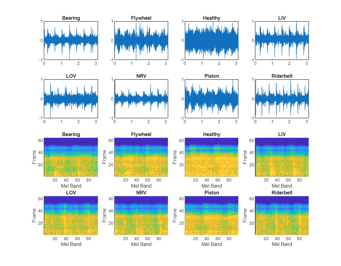
Extract Mel spectrograms for a sample recording of each class by using the yamnetPreprocess (Audio Toolbox) function. Each audio signal generates multiple Mel spectrograms. Display each sample recording and its first Mel spectrogram.
figure(Name="Imported Data",Units="Normalized",Position=[0.05, 0.25, 0.80, 1]);
for n = 1:numel(uniqueLabels)
    label = uniqueLabels(n);
    idx = find(ads.Labels==label,1);
    [x,fs] = audioread(ads.Files{idx});

    t = (0:size(x,1)-1)/fs;

    subplot(4,4,n);
    plot(t,x);
    title(label);

    melSpectYam = yamnetPreprocess(x,fs);
    melSpect = squeeze(melSpectYam(:,:,:,1));

    subplot(4,4,n+8);
    imagesc(CData=melSpect')
    axis([1 size(melSpect,2) 1 size(melSpect,1)])
    axis tight
    title(uniqueLabels(n));
    xlabel("Mel Band")
    ylabel("Frame")
end
Create Datastore of Spectrograms
Create a folder for each class label. These folders will store the Mel spectrograms that are used to train, calibrate, and test the anomaly detector.
spectDir = fullfile(pwd,"AirCompressorMelSpectrograms");
if ~exist(spectDir,"dir")
    mkdir(spectDir)
end
for n = 1:numel(uniqueLabels)
    labelDir = fullfile(spectDir,uniqueLabels(n));
    if ~exist(labelDir,"dir")
        mkdir(labelDir)
    end
end
Save the Mel spectrograms as JPG image files.
reset(ads)
k = 0;
while hasdata(ads)

    k = k+1;

    [audioIn,fileInfo] = read(ads);
    x = audioIn(:);
    fs = fileInfo.SampleRate;
    label = string(fileInfo.Label);

    melSpectYam = yamnetPreprocess(x,fs);
    melSpect = squeeze(melSpectYam(:,:,:,1));

    % Convert the spectrogram from a 2-D matrix to an RGB image with the
    % parula colormap
    im = ind2rgb(im2uint8(rescale(melSpect)),parula(256));
    % Resize as the network expects images to be at least 256-by-256 pixels
    im = imresize(im,4);
    imFilename = label+"_"+num2str(k,"%04d")+".jpg";
    imwrite(im,fullfile(spectDir,label,imFilename));
end
Manage access of the spectrogram images by using an imageDatastore. Specify the class labels as the folder names.
imds = imageDatastore(spectDir,IncludeSubfolders=true,LabelSource="foldernames");Partition Data
Define the labels for the normal class and the anomaly class. Normal images have the label "Healthy". Anomaly images have any other class label.
C = uniqueLabels(imds.Labels);
normalClass = "Healthy";
anomalyClasses = C(~ismember(C,normalClass));
This example trains the network using only normal images. Allocate 50% of the normal images for training. The example calibrates and tests the network using both normal and anomalous images. Allocate 20% each of normal and anomaly images for calibration, and allocate the rest of the data set for testing. To partition the data according to the target ratios, use the splitAnomalyData function.
normalTrainRatio  = 0.5;
anomalyTrainRatio = 0;
normalCalRatio  = 0.2;
anomalyCalRatio = 0.2;
normalTestRatio  = 1 - (normalTrainRatio + normalCalRatio);
anomalyTestRatio = 1 - (anomalyTrainRatio + anomalyCalRatio);

anomalyClasses = anomalyClasses(:)';  % Format anomalyClasses as a row vector
[imdsTrain,imdsCal,imdsTest] = splitAnomalyData(imds,anomalyClasses, ...
    NormalLabelsRatio=[normalTrainRatio normalCalRatio normalTestRatio], ...
    AnomalyLabelsRatio=[anomalyTrainRatio anomalyCalRatio anomalyTestRatio]);
Splitting anomaly dataset
-------------------------
* Finalizing... Done.
* Number of files and proportions per class in all the datasets:

                       Input                Train             Validation               Test
                 _________________    _________________    _________________    ___________________

                 NumFiles    Ratio    NumFiles    Ratio    NumFiles    Ratio    NumFiles     Ratio
                 ________    _____    ________    _____    ________    _____    ________    _______

    Bearing        225       0.125        0         0         45       0.125      180       0.13564
    Flywheel       225       0.125        0         0         45       0.125      180       0.13564
    Healthy        225       0.125      113         1         45       0.125       67       0.05049
    LIV            225       0.125        0         0         45       0.125      180       0.13564
    LOV            225       0.125        0         0         45       0.125      180       0.13564
    NRV            225       0.125        0         0         45       0.125      180       0.13564
    Piston         225       0.125        0         0         45       0.125      180       0.13564
    Riderbelt      225       0.125        0         0         45       0.125      180       0.13564
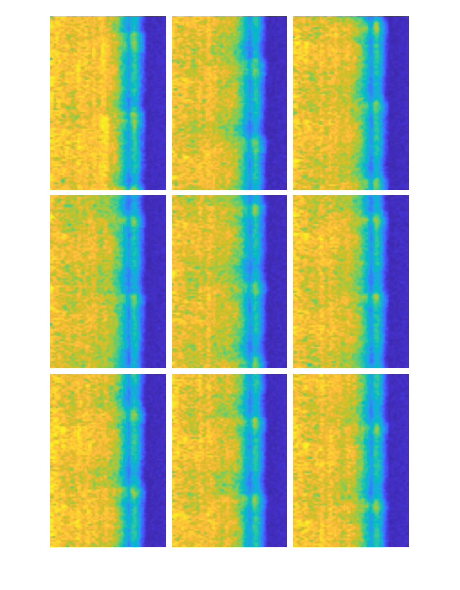
Read a subset of the training images and display them as a montage.
exampleData = readall(subset(imdsTrain,1:9));
figure
montage(exampleData(:,1),Size=[3 3], ...
    BorderSize=5,BackgroundColor="w");
Train Network or Download Pretrained Network
By default, this example downloads a pretrained version of the EfficientAD anomaly detector by using the helper function downloadTrainedNetwork. The function is attached to this example as a supporting file. You can use the pretrained network to calibrate and evaluate the model without waiting for training to complete.
To train the detector, set the doTraining variable in the following code to true. Create an untrained model by using the efficientADAnomalyDetector function. Train the model by using the trainEfficientADAnomalyDetector function.
Train on one or more GPUs, if they are available. Using a GPU requires a Parallel Computing Toolbox™ license and a CUDA®-enabled NVIDIA® GPU. For more information, see GPU Computing Requirements (Parallel Computing Toolbox).
doTraining =false; if doTraining % Define EfficientAD anomaly detector network architecture net = efficientADAnomalyDetector(Network="pdn-small"); % Configure training options maxEpochs = 60; lr = 1.5e-3; miniBatchSize = 16; l2reg = 1e-4; options = trainingOptions("adam",... InitialLearnRate = lr,... L2Regularization=l2reg,... LearnRateSchedule="piecewise",... LearnRateDropPeriod=floor(0.95*maxEpochs),... LearnRateDropFactor=0.1,... MaxEpochs=maxEpochs,... VerboseFrequency=2,... MiniBatchSize=miniBatchSize,... Shuffle="every-epoch",... ValidationData=dsCal,... ValidationPatience=Inf,... OutputNetwork="best-validation",... Metrics = aucMetric(Name="auc"),... ObjectiveMetricName = "auc",... ResetInputNormalization=true,... Plots="training-progress",... PreprocessingEnvironment="parallel"); detector = trainEfficientADAnomalyDetector(imdsTrain,net,options); modelDateTime = string(datetime("now",Format="yyyy-MM-dd-HH-mm-ss")); save(fullfile(tempdir,"trainedAirCompressorDefectDetectorEfficientAD_"+modelDateTime+".mat"), ... "detector"); else trainedAirCompressorDefectDetectorNetURL = "https://ssd.mathworks.com/supportfiles/"+ ... "vision/data/trainedAirCompressorDefectDetectorEfficientAD.zip"; downloadTrainedNetwork(trainedAirCompressorDefectDetectorNetURL,pwd); load("trainedAirCompressorDefectDetectorEfficientAD.mat"); end
Set Anomaly Threshold
After you train the EfficientAD detector or load a pretrained detector, you must set the anomaly score threshold for the detector. The detector classifies images based on whether their scores are above or below the threshold value. Calculate the anomaly threshold using the calibration images.
Predict the maximum anomaly score for each calibration image using the trained EfficientAD detector.
calScores = predict(detector,imdsCal);
Convert the ground truth labels of the calibration images into a binary classification. The label value 0 (false) corresponds to the normal ("Healthy") class. The label value 1 (true) corresponds to the anomaly class, which consists of all of the anomaly subclasses.
calLabels = imdsCal.Labels ~= "Healthy";Separate the anomaly scores into two variables. One vector stores the scores of normal images and the other vector stores the scores of the anomalous images.
calScoresNormal = calScores(calLabels==0);
calScoresAnomaly = calScores(calLabels==1);
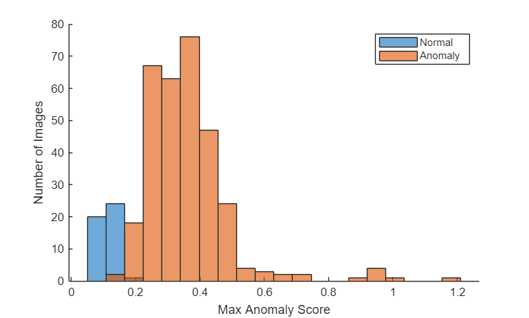
Plot a histogram of the anomaly scores for the normal and anomalous classes. The distributions are well separated by the model-predicted anomaly score.
numBins = 20;
[~,edges] = histcounts(calScores,numBins);
figure
hold on
hNormal = histogram(calScoresNormal,edges);
hAnomaly = histogram(calScoresAnomaly,edges);
hold off
legend([hNormal hAnomaly],"Normal","Anomaly")
xlabel("Max Anomaly Score")
ylabel("Number of Images")
Calculate the optimal anomaly threshold by using the anomalyThreshold function. Specify the first two input arguments as the binary ground truth labels and the predicted anomaly scores for the calibration images. Specify the third input argument as true because anomaly images have a label value of true. The anomalyThreshold function returns the optimal threshold value as a numeric scalar and the receiver operating characteristic (ROC) curve for the detector as an rocmetrics (Deep Learning Toolbox) object.
[thresh,roc] = anomalyThreshold(calLabels,calScores,true);
Set the Threshold property of the anomaly detector to the optimal value.
detector.Threshold = thresh;
Plot the ROC curve by using the plot (Deep Learning Toolbox) object function of rocmetrics. The ROC curve illustrates the performance of the classifier for a range of possible threshold values. Each point on the ROC curve represents the false positive rate (x-coordinate) and true positive rate (y-coordinate) when the calibration set images are classified using a different threshold value. The solid blue line represents the ROC curve. The area under the ROC curve (AUC) metric indicates classifier performance, and the maximum ROC AUC corresponding to a perfect classifier is 1.0.
plot(roc)
title("ROC AUC: "+ roc.AUC)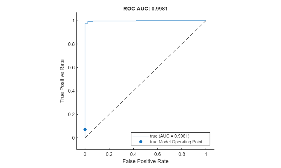
Evaluate Classification Model
Classify each test image as either normal or anomalous. The label value 0 (false) corresponds to the normal class. The label value 1 (true) corresponds to the anomaly class. The test images are full-size, which can cause out of memory errors on a GPU. To prevent out of memory errors, you can decrease the mini-batch size.
testLabelsPred = classify(detector,imdsTest);
testLabelsPred = testLabelsPred';
Get the ground truth labels for the test images. These ground truth labels are the subclass labels.
testSubclassLabelsGT = imdsTest.Labels;
To match the format of the predicted labels, convert the ground truth labels into a binary classification. Assign the value 0 (false) corresponds to the normal class and the value 1 (true) to any of the anomaly subclasses.
testLabelsGT = testSubclassLabelsGT ~= "Healthy";Calculate anomaly detection metrics by using the evaluateAnomalyDetection function. This function supports calculating the metrics of subclasses, so you can specify the ground truth labels as the anomaly subclass labels.
metrics = evaluateAnomalyDetection(testLabelsPred,testSubclassLabelsGT,anomalyClasses);
Evaluating anomaly detection results
------------------------------------
* Finalizing... Done.
* Data set metrics:

    GlobalAccuracy    MeanAccuracy    Precision    Recall     Specificity    F1Score    FalsePositiveRate    FalseNegativeRate
    ______________    ____________    _________    _______    ___________    _______    _________________    _________________

       0.97965          0.96809        0.99758     0.98095      0.95522      0.9892         0.044776             0.019048
Display the confusion matrix.
M = metrics.ConfusionMatrix{:,:};
confusionchart(M,["Normal" "Anomaly"])
acc = sum(diag(M)) / sum(M,"all");
title("Accuracy: "+acc)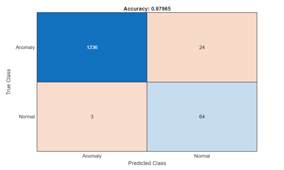
Display the accuracy of the normal and anomaly classes.
metrics.ClassMetrics
ans=2×2 table
               Accuracy    AccuracyPerSubClass
               ________    ___________________

    Normal     0.95522         {1×1 table}
    Anomaly    0.98095         {7×1 table}
Display the accuracy of subclasses within the anomaly class.
metrics.ClassMetrics(2,"AccuracyPerSubClass").AccuracyPerSubClass{1}ans=7×1 table
AccuracyPerSubClass
___________________
Bearing 0.98333
Flywheel 0.97222
LIV 1
LOV 0.93889
NRV 1
Piston 0.98333
Riderbelt 0.98889
Explain Classification Decisions
You can use the anomaly heatmap that the anomaly detector predicts to explain why the detector classifies an image as normal or anomalous. This approach is useful for identifying patterns in false negatives and false positives. You can use these patterns to identify strategies for increasing class balancing of the training data or improving the network performance.
Calculate a display range that reflects the range of anomaly scores observed across the entire calibration set, including normal and anomalous images. By using the same display range across images, you can compare images more easily than if you scale each image to its own minimum and maximum. Apply the display range to all heatmaps in this example.
minMapVal = inf;
maxMapVal = -inf;
reset(imdsCal)
while hasdata(imdsCal)
    img = read(imdsCal);
    map = anomalyMap(detector,img);
    minMapVal = min(min(map,[],"all"),minMapVal);
    maxMapVal = max(max(map,[],"all"),maxMapVal);
end
displayRange = [minMapVal 0.7*maxMapVal];
View Heatmap of Anomalous Image
A correctly classified anomaly, or true positive, is an image that is labeled as anomalous (1) by both the trained detector and the ground truth. Select a true positive image.
idxTruePositive = find(testLabelsGT & testLabelsPred);
img = readimage(imdsTest,idxTruePositive(1));
Calculate the heatmap of the image. Then, display an overlay of the heatmap on the image by using the anomalyMapOverlay function.
map = anomalyMap(detector,img);
imshow(anomalyMapOverlay(img,map,MapRange=displayRange,Blend="equal"))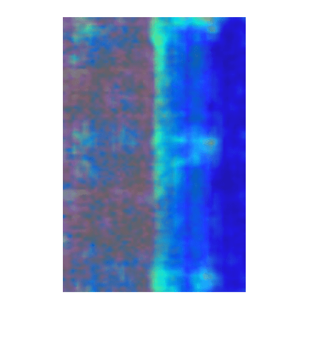
View Heatmap of Normal Image
A correctly classified normal image, or true negative, is an image that is labeled as normal (0) by both the trained detector and the ground truth. Select a true negative image.
idxTrueNegative = find(~testLabelsGT & ~testLabelsPred);
img = readimage(imdsTest,idxTrueNegative(1));
Calculate the heatmap of the image. Then, display an overlay of the heatmap on the image.
map = anomalyMap(detector,img);
imshow(anomalyMapOverlay(img,map,MapRange=displayRange,Blend="equal"))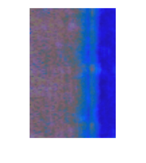
View Heatmap of False Positive Image
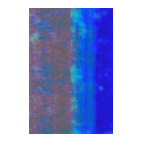
False positives are normal images that the network classifies as anomalous. For false positives, the ground truth label is 0 and the predicted label is 1. Select a false positive image, then calculate the heatmap of the image and display an overlay of the heatmap on the image.
Overlay the heatmap on the false positive image to gain insight into the misclassification. For this test image, anomalous scores are localized to image areas with uneven lightning. To decrease false positive results, you could adjust the image contrast during preprocessing, increase the number of images used for training, or choose a different threshold at the calibration step.
idxFalsePositive = find(~testLabelsGT & testLabelsPred);
if ~isempty(idxFalsePositive)
    img = readimage(imdsTest,idxFalsePositive(1));
    map = anomalyMap(detector,img);
    imshow(anomalyMapOverlay(img,map,MapRange=displayRange,Blend="equal"));
end
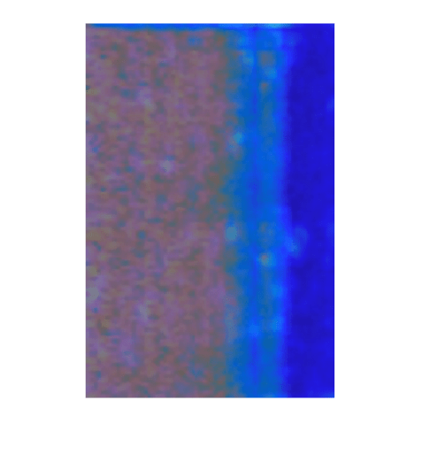
View Heatmap of False Negative Image
False negatives are images with defect anomalies that the network classifies as normal. For false negatives, the ground truth label is 1 and the predicted label is 0. Select a false negative image, then calculate the heatmap of the image.
Overlay the heatmap on the false negative image to gain insight into the misclassification. To decrease false negative results, consider adjusting the anomaly threshold of the detector.
idxFalseNegative = find(testLabelsGT & ~testLabelsPred);
if ~isempty(idxFalseNegative)
    img = readimage(imdsTest,idxFalseNegative(1));
    map = anomalyMap(detector,img);
    imshow(anomalyMapOverlay(img,map,MapRange=displayRange,Blend="equal"))
end
References
[1] Batzner, Kilian, Lars Heckler, and Rebecca König. "EfficientAD: Accurate Visual Anomaly Detection at Millisecond-Level Latencies." In Proceedings of the IEEE/CVF Winter Conference on Applications of Computer Vision, pp. 128–138. 2024. https://arxiv.org/abs/2303.14535.
[2] Verma, Nishchal K., Rahul Kumar Sevakula, Sonal Dixit, and Al Salour. “Intelligent Condition Based Monitoring Using Acoustic Signals for Air Compressors.” IEEE Transactions on Reliability 65, no. 1 (March 2016): 291–309. https://doi.org/10.1109/TR.2015.2459684.
See Also
trainEfficientADAnomalyDetector | efficientADAnomalyDetector | predict | anomalyMap | evaluateAnomalyDetection | trainingOptions (Deep Learning Toolbox) | anomalyThreshold | audioDatastore (Audio Toolbox) | yamnetPreprocess (Audio Toolbox)
Topics
- Getting Started with Anomaly Detection Using Deep Learning
- Acoustics-Based Machine Fault Recognition (Audio Toolbox)
- Deep Learning in MATLAB (Deep Learning Toolbox)
- Pretrained Deep Neural Networks (Deep Learning Toolbox)