gegenbauerC
Gegenbauer polynomials
Syntax
Description
gegenbauerC(
represents the n,a,x)nth-degree Gegenbauer
(ultraspherical) polynomial with parameter a at the point
x.
Examples
First Four Gegenbauer Polynomials
Find the first four Gegenbauer polynomials for the parameter
a and variable x.
syms a x
gegenbauerC([0, 1, 2, 3], a, x)
ans =
[ 1, 2*a*x, (2*a^2 + 2*a)*x^2 - a,...
((4*a^3)/3 + 4*a^2 + (8*a)/3)*x^3 + (- 2*a^2 - 2*a)*x]
Gegenbauer Polynomials for Numeric and Symbolic Arguments
Depending on its arguments, gegenbauerC returns
floating-point or exact symbolic results.
Find the value of the fifth-degree Gegenbauer polynomial for the parameter a =
1/3 at these points. Because these numbers are not symbolic objects,
gegenbauerC returns floating-point results.
gegenbauerC(5, 1/3, [1/6, 1/4, 1/3, 1/2, 2/3, 3/4])
ans =
    0.1520    0.1911    0.1914    0.0672   -0.1483   -0.2188
Find the value of the fifth-degree Gegenbauer polynomial for the same numbers converted
to symbolic objects. For symbolic numbers, gegenbauerC returns exact
symbolic results.
gegenbauerC(5, 1/3, sym([1/6, 1/4, 1/3, 1/2, 2/3, 3/4]))
ans =
[ 26929/177147, 4459/23328, 33908/177147, 49/729, -26264/177147, -7/32]
Evaluate Chebyshev Polynomials with Floating-Point Numbers
Floating-point evaluation of Gegenbauer polynomials by direct calls
of gegenbauerC is numerically stable. However, first computing the
polynomial using a symbolic variable, and then substituting variable-precision values into
this expression can be numerically unstable.
Find the value of the 500th-degree Gegenbauer polynomial for the parameter
4 at 1/3 and vpa(1/3).
Floating-point evaluation is numerically stable.
gegenbauerC(500, 4, 1/3)
gegenbauerC(500, 4, vpa(1/3))
ans =
  -1.9161e+05

ans =
-191609.10250897532784888518393655
Now, find the symbolic polynomial C500 = gegenbauerC(500, 4, x), and
substitute x = vpa(1/3) into the result. This approach is numerically
unstable.
syms x
C500 = gegenbauerC(500, 4, x);
subs(C500, x, vpa(1/3))
ans =
-8.0178726380235741521208852037291e+35
Approximate the polynomial coefficients by using vpa, and then
substitute x = sym(1/3) into the result. This approach is also
numerically unstable.
subs(vpa(C500), x, sym(1/3))
ans =
-8.1125412405858470246887213923167e+36
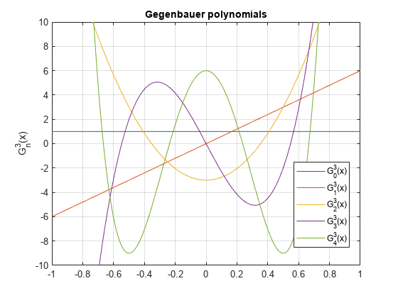
Plot Gegenbauer Polynomials
Plot the first five Gegenbauer polynomials for the parameter a = 3.
syms x y
fplot(gegenbauerC(0:4,3,x))
axis([-1 1 -10 10])
grid on

ylabel('G_n^3(x)')
title('Gegenbauer polynomials')
legend('G_0^3(x)', 'G_1^3(x)', 'G_2^3(x)', 'G_3^3(x)', 'G_4^3(x)',...
                                               'Location', 'Best')
Input Arguments
More About
Tips
gegenbauerCreturns floating-point results for numeric arguments that are not symbolic objects.gegenbauerCacts element-wise on nonscalar inputs.All nonscalar arguments must have the same size. If one or two input arguments are nonscalar, then
gegenbauerCexpands the scalars into vectors or matrices of the same size as the nonscalar arguments, with all elements equal to the corresponding scalar.
References
[1] Hochstrasser, U. W. “Orthogonal Polynomials.” Handbook of Mathematical Functions with Formulas, Graphs, and Mathematical Tables. (M. Abramowitz and I. A. Stegun, eds.). New York: Dover, 1972.
[2] Cohl, Howard S., and Connor MacKenzie. “Generalizations and Specializations of Generating Functions for Jacobi, Gegenbauer, Chebyshev and Legendre Polynomials with Definite Integrals.” Journal of Classical Analysis, no. 1 (2013): 17–33. https://doi.org/10.7153/jca-03-02.
Version History
Introduced in R2014b
See Also
chebyshevT | chebyshevU | hermiteH | jacobiP | laguerreL | legendreP