fairnessMetrics

Bias and group metrics for a data set or classification model

Since R2022b

Description

fairnessMetrics computes fairness metrics (bias and group metrics) for a data set or binary classification model with respect to sensitive attributes. The data-level evaluation examines binary, true labels of the data. The model-level evaluation examines the predicted labels returned by one or more binary classification models, using both true labels and predicted labels.

Bias metrics measure differences across groups, and group metrics contain information within the group. You can use the metrics to determine if your data or models contain bias toward a group within each sensitive attribute.

After creating a fairnessMetrics object, use the report function to generate a fairness metrics report or use the plot function to create a bar graph of the metrics.

Creation

Syntax

metricsResults = fairnessMetrics(SensitiveAttributes,Y)

metricsResults = fairnessMetrics(Tbl,Y)

metricsResults = fairnessMetrics(Tbl,ResponseName)

metricsResults = fairnessMetrics(___,SensitiveAttributeNames=sensitiveAttributeNames)

metricsResults = fairnessMetrics(___,Predictions=predictions)

metricsResults = fairnessMetrics(___,Name=Value)

Description

metricsResults = fairnessMetrics(SensitiveAttributes,Y) computes fairness metrics for the true, binary class labels in the vector Y with respect to the sensitive attributes in the SensitiveAttributes matrix. The fairnessMetrics function returns the fairnessMetrics object metricsResults, which stores bias metrics and group metrics in the BiasMetrics and GroupMetrics properties, respectively.

metricsResults = fairnessMetrics(Tbl,Y) computes fairness metrics using the sensitive attributes in the table Tbl and the class labels in the vector Y.

metricsResults = fairnessMetrics(Tbl,ResponseName) computes fairness metrics using the sensitive attributes and response variable in the table Tbl. The input argument ResponseName specifies the name of the variable in Tbl that contains the class labels.

metricsResults = fairnessMetrics(___,SensitiveAttributeNames=sensitiveAttributeNames) specifies a subset of the variables in Tbl (whose names correspond to sensitiveAttributeNames) as sensitive attributes, or assigns names to the sensitive attributes in sensitiveAttributeNames. You can specify this argument in addition to any of the input argument combinations in the previous syntaxes.

metricsResults = fairnessMetrics(___,Predictions=predictions) computes fairness metrics for one or more binary classification models when you specify each model's predicted labels by using the predictions argument. fairnessMetrics uses both true labels and predicted labels for the model-level evaluation.

metricsResults = fairnessMetrics(___,Name=Value) specifies additional options using one or more name-value arguments. For example, specify SensitiveAttributeNames="age",ReferenceGroup=30 to compute bias metrics for each group in the age variable with respect to the reference age group 30.

Input Arguments

SensitiveAttributes — Sensitive attributes

vector | matrix

Sensitive attributes, specified as a vector or matrix. If you specify SensitiveAttributes as a matrix, each row of SensitiveAttributes corresponds to one observation, and each column corresponds to one sensitive attribute.

You can use the sensitiveAttributeNames argument to assign names to the variables in SensitiveAttributes.

Data Types: single | double | logical | char | string | cell | categorical

Y — True, binary class labels

categorical array | character array | string array | logical vector | numeric vector | cell array of character vectors

True, binary class labels, specified as a categorical, character, or string array; a logical or numeric vector; or a cell array of character vectors.

• fairnessMetrics supports only binary classification. Y must contain exactly two distinct classes.

• You can specify one of the two classes as a positive class by using the PositiveClass name-value argument.

• The length of Y must be equal to the number of observations in SensitiveAttributes or Tbl.

• If Y is a character array, then each label must correspond to one row of the array.

Data Types: single | double | logical | char | string | cell | categorical

Tbl — Sample data

table

Sample data, specified as a table. Each row of Tbl corresponds to one observation, and each column corresponds to one sensitive attribute. Multicolumn variables and cell arrays other than cell arrays of character vectors are not allowed.

Optionally, Tbl can contain columns for the true class labels, predicted class labels, and observation weights.

• You must specify the true class label variable using ResponseName, the predicted class label variables using Predictions, and the observation weight variable using Weights. fairnessMetrics uses the remaining variables as sensitive attributes. To use a subset of the remaining variables in Tbl as sensitive attributes, specify the variables by using sensitiveAttributeNames.

• The true class label variable must be a categorical, character, or string array, a logical or numeric vector, or a cell array of character vectors.

  • fairnessMetrics supports only binary classification. The true class label variable must contain exactly two distinct classes.

  • You can specify one of the two classes as a positive class by using the PositiveClass name-value argument.

• The column for the weights must be a numeric vector.

If Tbl does not contain the true class label variable, then specify the variable by using Y. The length of the response variable Y and the number of rows in Tbl must be equal. To use a subset of the variables in Tbl as sensitive attributes, specify the variables by using sensitiveAttributeNames.

Data Types: table

ResponseName — Name of true class label variable

name of variable in Tbl

Name of the true class label variable, specified as a character vector or string scalar containing the name of the response variable in Tbl.

Example: "trueLabel" indicates that the trueLabel variable in Tbl (Tbl.trueLabel) is the true class label variable.

Data Types: char | string

sensitiveAttributeNames — Names of sensitive attribute variables

character vector | string array of unique names | cell array of unique character vectors

Names of the sensitive attribute variables, specified as a character vector, string array of unique names, or cell array of unique character vectors. The functionality of sensitiveAttributeNames depends on the way you supply the sample data.

• If you supply SensitiveAttributes and Y, then you can use sensitiveAttributeNames to assign names to the variables in SensitiveAttributes.

  • The order of the names in sensitiveAttributeNames must correspond to the column order of SensitiveAttributes. That is, sensitiveAttributeNames{1} is the name of SensitiveAttributes(:,1), sensitiveAttributeNames{2} is the name of SensitiveAttributes(:,2), and so on. Also, size(SensitiveAttributes,2) and numel(sensitiveAttributeNames) must be equal.

  • By default, sensitiveAttributeNames is {'x1','x2',...}.

• If you supply Tbl, then you can use sensitiveAttributeNames to specify the variables to use as sensitive attributes. That is, fairnessMetrics uses only the variables in sensitiveAttributeNames to compute fairness metrics.

  • sensitiveAttributeNames must be a subset of Tbl.Properties.VariableNames and cannot include the name of a class label variable or observation weight variable.

  • By default, sensitiveAttributeNames is a set of all variable names in Tbl, except the variables specified by ResponseName, Predictions, and Weights.

Example: SensitiveAttributeNames="Gender"

Example: SensitiveAttributeNames=["age","marital_status"]

Data Types: char | string | cell

predictions — Predicted class labels

[] (default) | names of variables in Tbl | matrix

Predicted class labels (model predictions), specified as [], the names of variables in Tbl, or a matrix.

Before R2023a: Specify predicted labels for at most one binary classifier by using the name of a variable in Tbl or a vector.

• [] — fairnessMetrics computes fairness metrics for the true class label variable (Y or the ResponseName variable in Tbl).

• Names of variables in Tbl — If you specify the input data as a table Tbl, then predictions can specify the name of one or more variables in Tbl, where each variable contains the predicted class labels for one model. In this case, you must specify predictions as a character vector, string array, or cell array of character vectors. For example, if the table contains one vector of class labels, stored as Tbl.Pred, then specify predictions as "Pred".

• Matrix — Each row of the matrix corresponds to a sample, and each column corresponds to one model's predicted class labels. The number of rows in predictions must be equal to the number of samples in Y or Tbl. The predicted class labels in predictions must be elements of the true class label variable, and predictions must have the same data type as the true class label variable.

Note

If you specify predicted labels for one or more binary classification models, fairnessMetrics computes fairness metrics for each model that returned predicted labels.

Example: Predictions="Pred"

Example: Predictions=["SVMPred","TreePred"]

Data Types: single | double | logical | char | string | cell | categorical

Name-Value Arguments

Specify optional pairs of arguments as Name1=Value1,...,NameN=ValueN, where Name is the argument name and Value is the corresponding value. Name-value arguments must appear after other arguments, but the order of the pairs does not matter.

Example: Predictions="P",Weights="W" specifies the variables P and W in the table Tbl as the model predictions and observation weights, respectively.

ModelNames — Names of models

character vector | string array of unique names | cell array of unique character vectors

Since R2023a

Names of the models with the predicted class labels predictions, specified as a character vector, string array of unique names, or cell array of unique character vectors.

• When predictions is an array of names in Tbl, the order of the names in ModelNames must correspond to the order of the names in predictions. That is, ModelNames{1} is the name of the model with predicted labels in the predictions{1} table variable, ModelNames{2} is the name of the model with predicted labels in the predictions{2} table variable, and so on. numel(ModelNames) and numel(predictions) must be equal. By default, the ModelNames value is equivalent to predictions.

• When predictions is a matrix, the order of the names in ModelNames must correspond to the column order of predictions. That is, ModelNames{1} is the name of the model with the predicted labels predictions(:,1), ModelNames{2} is the name of the model with the predicted labels predictions(:,2), and so on. numel(ModelNames) and size(predictions,2) must be equal. By default, the ModelNames value is {'Model1','Model2',...}.

• When predictions is [], the ModelNames value is 'Model1'.

  Note

  You cannot specify the ModelNames value when the predictions value is [].

Example: ModelNames="Ensemble"

Example: ModelNames=["SVM","Tree"]

Data Types: char | string | cell

PositiveClass — Label of positive class

scalar

Label of the positive class, specified as a scalar. PositiveClass must have the same data type as the true class label variable.

The default PositiveClass value is the second class of the binary labels, according to the order returned by the unique function with the "sorted" option specified for the true class label variable.

Example: PositiveClass=categorical(">50K")

Data Types: categorical | char | string | logical | single | double | cell

ReferenceGroup — Reference group

vector containing mode of each sensitive attribute (default) | numeric vector | string array | cell array

Reference group for each sensitive attribute, specified as a numeric vector, string array, or cell array. Each element in the ReferenceGroup value must have the same data type as the corresponding sensitive attribute. If the sensitive attributes have mixed types, specify ReferenceGroup as a cell array. The number of elements in the ReferenceGroup value must match the number of sensitive attributes.

The default ReferenceGroup value is a vector containing the mode of each sensitive attribute. The mode is the most frequently occurring value without taking into account observation weights.

Example: ReferenceGroup={30,categorical("Married-civ-spouse")}

Data Types: single | double | string | cell

Weights — Observation weights

vector of 1s (default) | vector of scalar values | name of variable in Tbl

Observation weights, specified as a vector of scalar values or the name of a variable in Tbl. The software weights the observations in each row of SensitiveAttributes or Tbl with the corresponding value in Weights. The size of Weights must equal the number of rows in SensitiveAttributes or Tbl.

If you specify the input data as a table Tbl, then Weights can be the name of a variable in Tbl that contains a numeric vector. In this case, you must specify Weights as a character vector or string scalar. For example, if the weights vector W is stored in Tbl.W, then specify Weights as "W".

Example: Weights="W"

Data Types: single | double | char | string

Properties

BiasMetrics — Bias metrics

Read-only: table

This property is read-only.

Bias metrics, specified as a table.

fairnessMetrics computes the bias metrics for each group in each sensitive attribute, compared to the reference group of the attribute.

Each row of BiasMetrics contains the bias metrics for a group in a sensitive attribute.

• For data-level evaluation, the first and second variables in BiasMetrics correspond to the sensitive attribute name (SensitiveAttributeNames column) and the group name (Groups column), respectively.

• For model-level evaluation, the first variable corresponds to the model name (ModelNames column). The second and third variables correspond to the sensitive attribute name and the group name, respectively.

The rest of the variables correspond to the bias metrics in this table.

Metric Name	Description	Evaluation Type
StatisticalParityDifference	Statistical parity difference (SPD)	Data-level or model-level evaluation
DisparateImpact	Disparate impact (DI)	Data-level or model-level evaluation
EqualOpportunityDifference	Equal opportunity difference (EOD)	Model-level evaluation
AverageAbsoluteOddsDifference	Average absolute odds difference (AAOD)	Model-level evaluation

The supported bias metrics depend on whether you specify predicted labels by using the Predictions argument when you create a fairnessMetrics object.

• Data-level evaluation — If you specify true labels and do not specify predicted labels, the BiasMetrics property contains only StatisticalParityDifference and DisparateImpact.

• Model-level evaluation — If you specify both true labels and predicted labels, the BiasMetrics property contains all metrics listed in the table.

For definitions of the bias metrics, see Bias Metrics.

Data Types: table

GroupMetrics — Group metrics

Read-only: table

This property is read-only.

Group metrics, specified as a table.

The fairnessMetrics function computes the group metrics for each group in each sensitive attribute. Note that the function does not use the observation weights (specified by the Weights name-value argument) to count the number of samples in each group (GroupCount value). The function uses Weights to compute the other metrics.

Each row of GroupMetrics contains the group metrics for a group in a sensitive attribute.

• For data-level evaluation, the first and second variables in GroupMetrics correspond to the sensitive attribute name (SensitiveAttributeNames column) and the group name (Groups column), respectively.

• For model-level evaluation, the first variable corresponds to the model name (ModelNames column). The second and third variables correspond to the sensitive attribute name and the group name, respectively.

The rest of the variables correspond to the group metrics in this table.

Metric Name	Description	Evaluation Type
GroupCount	Group count, or number of samples in the group	Data-level or model-level evaluation
GroupSizeRatio	Group count divided by the total number of samples	Data-level or model-level evaluation
TruePositives	Number of true positives (TP)	Model-level evaluation
TrueNegatives	Number of true negatives (TN)	Model-level evaluation
FalsePositives	Number of false positives (FP)	Model-level evaluation
FalseNegatives	Number of false negatives (FN)	Model-level evaluation
TruePositiveRate	True positive rate (TPR), also known as recall or sensitivity, TP/(TP+FN)	Model-level evaluation
TrueNegativeRate	True negative rate (TNR), or specificity, TN/(TN+FP)	Model-level evaluation
FalsePositiveRate	False positive rate (FPR), also known as fallout or 1-specificity, FP/(TN+FP)	Model-level evaluation
FalseNegativeRate	False negative rate (FNR), or miss rate, FN/(TP+FN)	Model-level evaluation
FalseDiscoveryRate	False discovery rate (FDR), FP/(TP+FP)	Model-level evaluation
FalseOmissionRate	False omission rate (FOR), FN/(TN+FN)	Model-level evaluation
PositivePredictiveValue	Positive predictive value (PPV), or precision, TP/(TP+FP)	Model-level evaluation
NegativePredictiveValue	Negative predictive value (NPV), TN/(TN+FN)	Model-level evaluation
RateOfPositivePredictions	Rate of positive predictions (RPP), (TP+FP)/(TP+FN+FP+TN)	Model-level evaluation
RateOfNegativePredictions	Rate of negative predictions (RNP), (TN+FN)/(TP+FN+FP+TN)	Model-level evaluation
Accuracy	Accuracy, (TP+TN)/(TP+FN+FP+TN)	Model-level evaluation

The supported group metrics depend on whether you specify predicted labels by using the Predictions argument when you create a fairnessMetrics object.

• Data-level evaluation — If you specify true labels and do not specify predicted labels, the GroupMetrics property contains only GroupCount and GroupSizeRatio.

• Model-level evaluation — If you specify both true labels and predicted labels, the GroupMetrics property contains all metrics listed in the table.

Data Types: table

ModelNames — Names of models

Read-only: character vector | cell array of unique character vectors

Since R2023a

This property is read-only.

Names of the models with the predicted class labels predictions, specified as a character vector or cell array of unique character vectors. (The software treats string arrays as cell arrays of character vectors.)

The ModelNames name-value argument sets this property.

Data Types: char | cell

PositiveClass — Label of positive class

Read-only: scalar

This property is read-only.

Label of the positive class, specified as a scalar. (The software treats a string scalar as a character vector.)

The PositiveClass name-value argument sets this property.

Data Types: categorical | char | logical | single | double | cell

ReferenceGroup — Reference group

Read-only: numeric vector | cell array

This property is read-only.

Reference group, specified as a numeric vector or cell array. (The software treats string arrays as cell arrays of character vectors.)

The ReferenceGroup name-value argument sets this property.

Data Types: single | double | cell

ResponseName — Name of true class label variable

Read-only: character vector

This property is read-only.

Name of the true class label variable, specified as a character vector containing the name of the response variable. (The software treats a string scalar as a character vector.)

• If you specify the ResponseName argument, then the specified value determines this property.

• If you specify Y, then the property value is 'Y'.

Data Types: char

SensitiveAttributeNames — Names of sensitive attribute variables

Read-only: character vector | cell array of unique character vectors

This property is read-only.

Names of the sensitive attribute variables, specified as a character vector or cell array of unique character vectors. (The software treats string arrays as cell arrays of character vectors.)

The sensitiveAttributeNames argument sets this property.

Data Types: char | cell

Object Functions

report	Generate fairness metrics report
plot	Plot bar graph of fairness metric

Examples

Evaluate Fairness of Data

Compute fairness metrics for true labels with respect to sensitive attributes by creating a fairnessMetrics object. Then, create a table of fairness metrics by using the report function, and plot bar graphs of the metrics by using the plot function.

Load the sample data census1994, which contains the training data adultdata and the test data adulttest. The data sets consist of demographic information from the US Census Bureau that can be used to predict whether an individual makes over $50,000 per year. Preview the first few rows of the training data set.

load census1994
head(adultdata)

    age       workClass          fnlwgt      education    education_num       marital_status           occupation        relationship     race      sex      capital_gain    capital_loss    hours_per_week    native_country    salary
    ___    ________________    __________    _________    _____________    _____________________    _________________    _____________    _____    ______    ____________    ____________    ______________    ______________    ______

    39     State-gov                77516    Bachelors         13          Never-married            Adm-clerical         Not-in-family    White    Male          2174             0                40          United-States     <=50K 
    50     Self-emp-not-inc         83311    Bachelors         13          Married-civ-spouse       Exec-managerial      Husband          White    Male             0             0                13          United-States     <=50K 
    38     Private             2.1565e+05    HS-grad            9          Divorced                 Handlers-cleaners    Not-in-family    White    Male             0             0                40          United-States     <=50K 
    53     Private             2.3472e+05    11th               7          Married-civ-spouse       Handlers-cleaners    Husband          Black    Male             0             0                40          United-States     <=50K 
    28     Private             3.3841e+05    Bachelors         13          Married-civ-spouse       Prof-specialty       Wife             Black    Female           0             0                40          Cuba              <=50K 
    37     Private             2.8458e+05    Masters           14          Married-civ-spouse       Exec-managerial      Wife             White    Female           0             0                40          United-States     <=50K 
    49     Private             1.6019e+05    9th                5          Married-spouse-absent    Other-service        Not-in-family    Black    Female           0             0                16          Jamaica           <=50K 
    52     Self-emp-not-inc    2.0964e+05    HS-grad            9          Married-civ-spouse       Exec-managerial      Husband          White    Male             0             0                45          United-States     >50K  

Each row contains the demographic information for one adult. The information includes sensitive attributes, such as age, marital_status, relationship, race, and sex. The third column flnwgt contains observation weights, and the last column salary shows whether a person has a salary less than or equal to $50,000 per year (<=50K) or greater than $50,000 per year (>50K).

This example evaluates the fairness of the salary variable with respect to age. Group the age variable into four bins.

ageGroups = ["Age<30","30<=Age<45","45<=Age<60","Age>=60"];
adultdata.age_group = discretize(adultdata.age, ...
    [min(adultdata.age) 30 45 60 max(adultdata.age)], ...
    categorical=ageGroups);

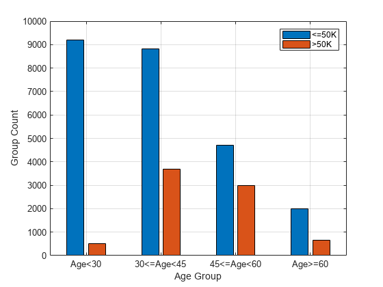
Plot the counts of individuals in each class (<=50K and >50K) by age.

figure
gc = groupcounts(adultdata,["age_group","salary"]);
bar([gc.GroupCount(1:2:end),gc.GroupCount(2:2:end)])
xticklabels(ageGroups)
xlabel("Age Group")
ylabel("Group Count")
legend(["<=50K",">50K"])
grid on

Compute fairness metrics for the salary variable with respect to the age_group variable by using fairnessMetrics.

metricsResults = fairnessMetrics(adultdata,"salary", ...
    SensitiveAttributeNames="age_group",Weights="fnlwgt")

metricsResults = 
  fairnessMetrics with properties:

    SensitiveAttributeNames: 'age_group'
             ReferenceGroup: '30<=Age<45'
               ResponseName: 'salary'
              PositiveClass: >50K
                BiasMetrics: [4×4 table]
               GroupMetrics: [4×4 table]


  Properties, Methods

metricsResults is a fairnessMetrics object. By default, the fairnessMetrics function selects the majority group of the sensitive attribute (group with the largest number of individuals) as the reference group for the attribute. Also, the fairnessMetrics function orders the labels by using the unique function with the "sorted" option, and specifies the second class of the labels as the positive class. In this data set, the reference group of age_group is the group 30<=Age<45, and the positive class is >50K. The object stores bias metrics and group metrics in the BiasMetrics and GroupMetrics properties, respectively. Display the properties.

metricsResults.BiasMetrics

ans=4×4 table
    SensitiveAttributeNames      Groups      StatisticalParityDifference    DisparateImpact
    _______________________    __________    ___________________________    _______________

           age_group           Age<30                 -0.24365                  0.17661    
           age_group           30<=Age<45                    0                        1    
           age_group           45<=Age<60             0.098497                   1.3329    
           age_group           Age>=60                -0.05041                  0.82965    

metricsResults.GroupMetrics

ans=4×4 table
    SensitiveAttributeNames      Groups      GroupCount    GroupSizeRatio
    _______________________    __________    __________    ______________

           age_group           Age<30           9711           0.29824   
           age_group           30<=Age<45      12489           0.38356   
           age_group           45<=Age<60       7717             0.237   
           age_group           Age>=60          2644          0.081201   

According to the bias metrics, the salary variable is biased toward the age group 45 to 60 years and biased against the age group less than 30 years, compared to the reference group (30<=Age<45).

You can create a table that contains both bias metrics and group metrics by using the report function. Specify GroupMetrics as "all" to include all group metrics. You do not have to specify the BiasMetrics name-value argument because its default value is "all".

metricsTbl = report(metricsResults,GroupMetrics="all")

metricsTbl=4×6 table
    SensitiveAttributeNames      Groups      StatisticalParityDifference    DisparateImpact    GroupCount    GroupSizeRatio
    _______________________    __________    ___________________________    _______________    __________    ______________

           age_group           Age<30                 -0.24365                  0.17661           9711           0.29824   
           age_group           30<=Age<45                    0                        1          12489           0.38356   
           age_group           45<=Age<60             0.098497                   1.3329           7717             0.237   
           age_group           Age>=60                -0.05041                  0.82965           2644          0.081201   

Visualize the bias metrics by using the plot function.

figure
t = tiledlayout(2,1);
nexttile
plot(metricsResults,"spd")
xlabel("")
ylabel("")
nexttile
plot(metricsResults,"di")
xlabel("")
ylabel("")
xlabel(t,"Fairness Metric Value")
ylabel(t,"Age Group")

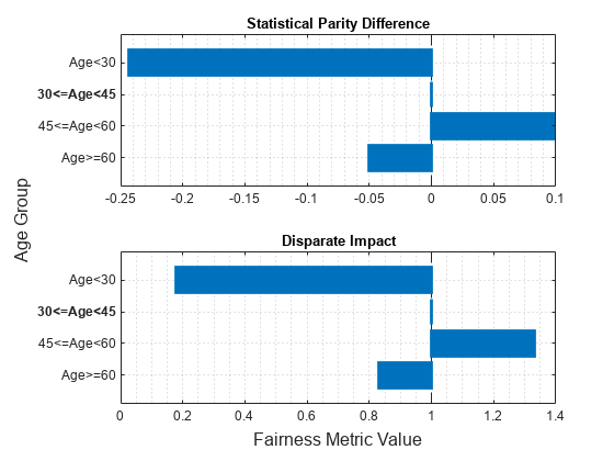
The vertical line in each plot ($$x=0$$ for statistical parity difference and $$x=1$$ for disparate impact) indicates the metric value for the reference group. If the labels do not have a bias for a target group compared to the reference group, the metric value for the target group is the same as the metric value for the reference group.

Evaluate Fairness of Classifier

Compute fairness metrics for predicted labels with respect to sensitive attributes by creating a fairnessMetrics object. Then, create a table of fairness metrics by using the report function, and plot bar graphs of the metrics by using the plot function.

Load the sample data census1994, which contains the training data adultdata and the test data adulttest. The data sets consist of demographic information from the US Census Bureau that can be used to predict whether an individual makes over $50,000 per year. Preview the first few rows of the training data set.

load census1994
head(adultdata)

    age       workClass          fnlwgt      education    education_num       marital_status           occupation        relationship     race      sex      capital_gain    capital_loss    hours_per_week    native_country    salary
    ___    ________________    __________    _________    _____________    _____________________    _________________    _____________    _____    ______    ____________    ____________    ______________    ______________    ______

    39     State-gov                77516    Bachelors         13          Never-married            Adm-clerical         Not-in-family    White    Male          2174             0                40          United-States     <=50K 
    50     Self-emp-not-inc         83311    Bachelors         13          Married-civ-spouse       Exec-managerial      Husband          White    Male             0             0                13          United-States     <=50K 
    38     Private             2.1565e+05    HS-grad            9          Divorced                 Handlers-cleaners    Not-in-family    White    Male             0             0                40          United-States     <=50K 
    53     Private             2.3472e+05    11th               7          Married-civ-spouse       Handlers-cleaners    Husband          Black    Male             0             0                40          United-States     <=50K 
    28     Private             3.3841e+05    Bachelors         13          Married-civ-spouse       Prof-specialty       Wife             Black    Female           0             0                40          Cuba              <=50K 
    37     Private             2.8458e+05    Masters           14          Married-civ-spouse       Exec-managerial      Wife             White    Female           0             0                40          United-States     <=50K 
    49     Private             1.6019e+05    9th                5          Married-spouse-absent    Other-service        Not-in-family    Black    Female           0             0                16          Jamaica           <=50K 
    52     Self-emp-not-inc    2.0964e+05    HS-grad            9          Married-civ-spouse       Exec-managerial      Husband          White    Male             0             0                45          United-States     >50K  

Each row contains the demographic information for one adult. The information includes sensitive attributes, such as age, marital_status, relationship, race, and sex. The third column flnwgt contains observation weights, and the last column salary shows whether a person has a salary less than or equal to $50,000 per year (<=50K) or greater than $50,000 per year (>50K).

Train a classification tree using the training data set adultdata. Specify the response variable, predictor variables, and observation weights by using the variable names in the adultdata table.

predictorNames = ["capital_gain","capital_loss","education", ...
    "education_num","hours_per_week","occupation","workClass"];
Mdl = fitctree(adultdata,"salary", ...
    PredictorNames=predictorNames,Weights="fnlwgt");

Predict the test sample labels by using the trained tree Mdl.

labels = predict(Mdl,adulttest);

This example evaluates the fairness of the predicted labels with respect to age and marital status. Group the age variable into four bins.

ageGroups = ["Age<30","30<=Age<45","45<=Age<60","Age>=60"];
adulttest.age_group = discretize(adulttest.age, ...
    [min(adulttest.age) 30 45 60 max(adulttest.age)], ...
    categorical=ageGroups);

Plot the counts of individuals in each predicted class (<=50K and >50K) by age.

figure
gs_age = groupcounts({adulttest.age_group,labels});
b_age = bar([gs_age(1:2:end),gs_age(2:2:end)]);
xticklabels(ageGroups)
xlabel("Age Group")
ylabel("Group Count")
legend(["<=50K",">50K"])
grid minor

Plot the counts of individuals by marital status. Display the count values near the tips of the bars if the values are smaller than 100.

figure
gs_status = groupcounts({adulttest.marital_status,labels});
b_status = bar([gs_status(1:2:end),gs_status(2:2:end)]);
xticklabels(unique(adulttest.marital_status))
xlabel("Marital Status")
ylabel("Group Count")
legend(["<=50K",">50K"])
grid minor

xtips1 = b_status(1).XEndPoints;
ytips1 = b_status(1).YEndPoints;
labels1 = string(b_status(1).YData);
ind1 = ytips1 < 100;
text(xtips1(ind1),ytips1(ind1),labels1(ind1), ...
    HorizontalAlignment="center",VerticalAlignment="bottom", ...
    Color=b_status(1).FaceColor)
xtips2 = b_status(2).XEndPoints;
ytips2 = b_status(2).YEndPoints;
labels2 = string(b_status(2).YData);
ind2 = ytips2 < 100;
text(xtips2(ind2),ytips2(ind2),labels2(ind2), ...
    HorizontalAlignment="center",VerticalAlignment="bottom", ...
    Color=b_status(2).FaceColor)

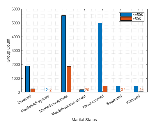
Compute fairness metrics for the predictions (labels) with respect to the age_group and marital_status variables by using fairnessMetrics.

metricsResults = fairnessMetrics(adulttest,"salary", ...
    SensitiveAttributeNames=["age_group","marital_status"], ...
    Predictions=labels,Weights="fnlwgt")

metricsResults = 
  fairnessMetrics with properties:

    SensitiveAttributeNames: {'age_group'  'marital_status'}
             ReferenceGroup: {'30<=Age<45'  'Married-civ-spouse'}
               ResponseName: 'salary'
              PositiveClass: >50K
                BiasMetrics: [11×7 table]
               GroupMetrics: [11×20 table]
                 ModelNames: 'Model1'


  Properties, Methods

metricsResults is a fairnessMetrics object. By default, the fairnessMetrics function selects the majority group of each sensitive attribute (group with the largest number of individuals) as the reference group for the attribute. Also, the fairnessMetrics function orders the labels by using the unique function with the "sorted" option, and specifies the second class of the labels as the positive class. In this data set, the reference groups of age_group and marital_status are the groups 30<=Age<45 and Married-civ-spouse, respectively, and the positive class is >50K. The object stores bias metrics and group metrics in the BiasMetrics and GroupMetrics properties, respectively.

Create a table with fairness metrics by using the report function. Specify BiasMetrics as ["eod","aaod"] to include the equal opportunity difference (EOD) and average absolute odds difference (AAOD) metrics in the report table. The fairnessMetrics function computes the two metrics by using the true positive rates (TPR) and false positive rates (FPR). Specify GroupMetrics as ["tpr","fpr"] to include TPR and FPR values in the table.

metricsTbl = report(metricsResults, ...
    BiasMetrics=["eod","aaod"],GroupMetrics=["tpr","fpr"])

metricsTbl=11×7 table
    ModelNames    SensitiveAttributeNames           Groups            EqualOpportunityDifference    AverageAbsoluteOddsDifference    TruePositiveRate    FalsePositiveRate
    __________    _______________________    _____________________    __________________________    _____________________________    ________________    _________________

      Model1          age_group              Age<30                           -0.041319                       0.044114                   0.41333             0.041709     
      Model1          age_group              30<=Age<45                               0                              0                   0.45465             0.088618     
      Model1          age_group              45<=Age<60                        0.061495                       0.031809                   0.51614             0.086495     
      Model1          age_group              Age>=60                          0.0060387                       0.011955                   0.46069             0.070746     
      Model1          marital_status         Divorced                          0.078541                       0.043643                   0.54263             0.075653     
      Model1          marital_status         Married-AF-spouse                 0.073166                       0.078782                   0.53726                    0     
      Model1          marital_status         Married-civ-spouse                       0                              0                   0.46409             0.084398     
      Model1          marital_status         Married-spouse-absent            -0.067098                       0.048093                   0.39699             0.055311     
      Model1          marital_status         Never-married                       0.0886                       0.057557                   0.55269             0.057883     
      Model1          marital_status         Separated                         0.027256                       0.026751                   0.49135             0.058151     
      Model1          marital_status         Widowed                            0.12442                       0.080073                   0.58851             0.048675     

Plot the EOD and AAOD values for the sensitive attribute age_group. Because age_group is the first element in the SensitiveAttributeNames property of metricsResults, it is the default value for the property. Therefore, you do not have to specify the SensitiveAttributeName argument of the plot function.

figure
t = tiledlayout(1,2);
nexttile
plot(metricsResults,"eod")
title("EOD")
xlabel("")
ylabel("")
nexttile
plot(metricsResults,"aaod")
title("AAOD")
xlabel("")
ylabel("")
yticklabels("")
xlabel(t,"Fairness Metric Value")
ylabel(t,"Age Group")

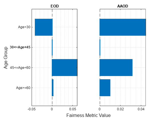
The vertical line at $$x=0$$ indicates the metric value for the reference group (30<=Age<45). If the labels do not have a bias for a target group compared to the reference group, the metric value for the target group is the same as the metric value for the reference group. According to the EOD values (differences in TPR), the predictions for the salary variable are most biased toward the group 45<=Age<60 compared to the reference group. According to the AAOD values (averaged differences in TPR and FPR), the predictions are most biased toward the group Age<30.

Plot the EOD and AAOD values for the sensitive attribute marital_status by specifying the SensitiveAttributeName argument of the plot function as marital_status.

figure
t = tiledlayout(1,2);
nexttile
plot(metricsResults,"eod",SensitiveAttributeName="marital_status")
title("EOD")
xlabel("")
ylabel("")
nexttile
plot(metricsResults,"aaod",SensitiveAttributeName="marital_status")
title("AAOD")
xlabel("")
ylabel("")
yticklabels("")
xlabel(t,"Fairness Metric Value")
ylabel(t,"Marital Status")

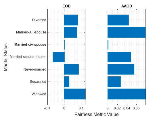
The vertical line at $$x=0$$ indicates the metric value for the reference group (Married-civ-spouse). According to the EOD values, the predictions for the salary variable are most biased toward the group Widowed compared to the reference group. According to the AAOD values, the predictions are similarly biased toward the groups Widowed and Married-AF-spouse.

Compare Model Predictions Using Fairness Metrics

Train two classification models, and compare the model predictions by using fairness metrics.

Read the sample file CreditRating_Historical.dat into a table. The predictor data consists of financial ratios and industry sector information for a list of corporate customers. The response variable consists of credit ratings assigned by a rating agency.

creditrating = readtable("CreditRating_Historical.dat");

Because each value in the ID variable is a unique customer ID—that is, length(unique(creditrating.ID)) is equal to the number of observations in creditrating—the ID variable is a poor predictor. Remove the ID variable from the table, and convert the Industry variable to a categorical variable.

creditrating.ID = [];
creditrating.Industry = categorical(creditrating.Industry);

In the Rating response variable, combine the AAA, AA, A, and BBB ratings into a category of "good" ratings, and the BB, B, and CCC ratings into a category of "poor" ratings.

Rating = categorical(creditrating.Rating);
Rating = mergecats(Rating,["AAA","AA","A","BBB"],"good");
Rating = mergecats(Rating,["BB","B","CCC"],"poor");
creditrating.Rating = Rating;

Train a support vector machine (SVM) model on the creditrating data. For better results, standardize the predictors before fitting the model. Use the trained model to predict labels and compute the misclassification rate for the training data set.

predictorNames = ["WC_TA","RE_TA","EBIT_TA","MVE_BVTD","S_TA"];
SVMMdl = fitcsvm(creditrating,"Rating", ...
    PredictorNames=predictorNames,Standardize=true);
SVMPredictions = resubPredict(SVMMdl);
resubLoss(SVMMdl)

ans = 
0.0872

Train a generalized additive model (GAM).

GAMMdl = fitcgam(creditrating,"Rating", ...
    PredictorNames=predictorNames);
GAMPredictions = resubPredict(GAMMdl);
resubLoss(GAMMdl)

ans = 
0.0542

GAMMdl achieves better accuracy on the training data set.

Compute fairness metrics with respect to the sensitive attribute Industry by using the model predictions for both models.

predictions = [SVMPredictions,GAMPredictions];
metricsResults = fairnessMetrics(creditrating,"Rating", ...
    SensitiveAttributeNames="Industry",Predictions=predictions, ...
    ModelNames=["SVM","GAM"]);

Display the bias metrics by using the report function.

report(metricsResults)

ans=48×5 table
              Metrics              SensitiveAttributeNames    Groups       SVM          GAM    
    ___________________________    _______________________    ______    _________    __________

    StatisticalParityDifference           Industry              1       -0.028441     0.0058208
    StatisticalParityDifference           Industry              2        -0.04014     0.0063339
    StatisticalParityDifference           Industry              3               0             0
    StatisticalParityDifference           Industry              4        -0.04905    -0.0043007
    StatisticalParityDifference           Industry              5       -0.015615     0.0041607
    StatisticalParityDifference           Industry              6        -0.03818     -0.024515
    StatisticalParityDifference           Industry              7        -0.01514      0.007326
    StatisticalParityDifference           Industry              8       0.0078632      0.036581
    StatisticalParityDifference           Industry              9       -0.013863      0.042266
    StatisticalParityDifference           Industry              10      0.0090218      0.050095
    StatisticalParityDifference           Industry              11      -0.004188      0.001453
    StatisticalParityDifference           Industry              12      -0.041572     -0.028589
    DisparateImpact                       Industry              1         0.92261         1.017
    DisparateImpact                       Industry              2         0.89078        1.0185
    DisparateImpact                       Industry              3               1             1
    DisparateImpact                       Industry              4         0.86654       0.98742
      ⋮

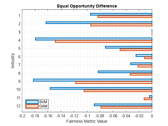
Among the bias metrics, compare the equal opportunity difference (EOD) values. Create a bar graph of the EOD values by using the plot function.

b = plot(metricsResults,"eod");
b(1).FaceAlpha = 0.2;
b(2).FaceAlpha = 0.2;
legend(Location="southwest")

To better understand the distributions of EOD values, plot the values using box plots.

boxchart(metricsResults.BiasMetrics.EqualOpportunityDifference, ...
    GroupByColor=metricsResults.BiasMetrics.ModelNames)
ax = gca;
ax.XTick = [];
ylabel("Equal Opportunity Difference")
legend

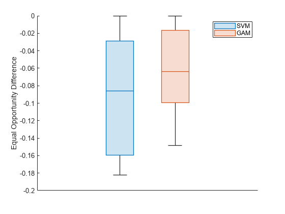
The EOD values for GAM are closer to 0 compared to the values for SVM.

More About

Bias Metrics

The fairnessMetrics object supports four bias metrics: statistical parity difference (SPD), disparate impact (DI), equal opportunity difference (EOD), and average absolute odds difference (AAOD). The object supports EOD and AAOD only for evaluating model predictions.

A fairnessMetrics object computes bias metrics for each group in each sensitive attribute with respect to the reference group of the attribute.

• Statistical parity (or demographic parity) difference (SPD)

  The SPD value of the ith sensitive attribute (S_i) for the group s_ij with respect to the reference group s_ir is defined by

  $${\text{SPD}}_{ij}=P\left(Y=+|S_i=s_{ij}\right)-P\left(Y=+|S_i=s_{ir}\right).$$

  The SPD value is the difference between the probability of being in the positive class when the sensitive attribute value is s_ij and the probability of being in the positive class when the sensitive attribute value is s_ir (reference group). This metric assumes that the two probabilities (statistical parities) are equal if the labels are unbiased with respect to the sensitive attribute.

  If you specify the Predictions argument, the software computes SPD for the probabilities of the model predictions $$\widehat{Y}$$ instead of the true labels Y.

• Disparate impact (DI)

  The DI value of the ith sensitive attribute (S_i) for the group s_ij with respect to the reference group s_ir is defined by

  $${\text{DI}}_{ij}=\frac{P\left(Y=+|S_i=s_{ij}\right)}{P\left(Y=+|S_i=s_{ir}\right)}.$$

  The DI value is the ratio of the probability of being in the positive class when the sensitive attribute value is s_ij to the probability of being in the positive class when the sensitive attribute value is s_ir (reference group). This metric assumes that the two probabilities are equal if the labels are unbiased with respect to the sensitive attribute. In general, a DI value less than 0.8 or greater than 1.25 indicates bias with respect to the reference group [2].

  If you specify the Predictions argument, the software computes DI for the probabilities of the model predictions $$\widehat{Y}$$ instead of the true labels Y.

• Equal opportunity difference (EOD)

  The EOD value of the ith sensitive attribute (S_i) for the group s_ij with respect to the reference group s_ir is defined by

  $$\begin{array}{c}{\text{EOD}}_{ij}=\text{TPR}\left(S_i=s_{ij}\right)-\text{TPR}\left(S_i=s_{ir}\right)\\ =P\left(\widehat{Y}=+|Y=+,S_i=s_{ij}\right)-P\left(\widehat{Y}=+|Y=+,S_i=s_{ir}\right).\end{array}$$

  The EOD value is the difference in the true positive rate (TPR) between the group s_ij and the reference group s_ir. This metric assumes that the two rates are equal if the predicted labels are unbiased with respect to the sensitive attribute.

• Average absolute odds difference (AAOD)

  The AAOD value of the ith sensitive attribute (S_i) for the group s_ij with respect to the reference group s_ir is defined by

  $${\text{AAOD}}_{ij}=\frac{1}{2}\left(\left|\text{FPR}\left(S_i=s_{ij}\right)-\text{FPR}\left(S_i=s_{ir}\right)\right|+\left|\text{TPR}\left(S_i=s_{ij}\right)-\text{TPR}\left(S_i=s_{ir}\right)\right|\right).$$

  The AAOD value represents the difference in the true positive rates (TPR) and false positive rates (FPR) between the group s_ij and the reference group s_ir. This metric assumes no difference in TPR and FPR if the predicted labels are unbiased with respect to the sensitive attribute.

Algorithms

fairnessMetrics considers NaN, '' (empty character vector), "" (empty string), <missing>, and <undefined> values in Tbl, Y, and SensitiveAttributes to be missing values. fairnessMetrics does not use observations with missing values.

References

[1] Mehrabi, Ninareh, et al. “A Survey on Bias and Fairness in Machine Learning.” ArXiv:1908.09635 [cs.LG], Sept. 2019. arXiv.org.

[2] Saleiro, Pedro, et al. “Aequitas: A Bias and Fairness Audit Toolkit.” ArXiv:1811.05577 [cs.LG], April 2019. arXiv.org.

Version History

Introduced in R2022b

R2023a: Compare fairness metrics across models

You can compare fairness metrics across multiple binary classifiers by using the fairnessMetrics function. In the call to the function, use the predictions argument and specify the predicted class labels for each model. To specify the names of the models, you can use the ModelNames name-value argument. The model name information is stored in the BiasMetrics, GroupMetrics, and ModelNames properties of the fairnessMetrics object.

After you create a fairnessMetrics object, use the report or plot object function.

• The report object function returns a fairness metrics table, whose format depends on the value of the DisplayMetricsInRows name-value argument. (For more information, see metricsTbl.) You can specify a subset of models to include in the report table by using the ModelNames name-value argument.

• The plot object function returns a bar graph as an array of Bar objects. The bar colors indicate the models whose predicted labels are used to compute the specified metric. You can specify a subset of models to include in the plot by using the ModelNames name-value argument.

In previous releases, the first and second variables in the BiasMetrics and GroupMetrics properties of the fairnessMetrics object always corresponded to the sensitive attribute name (SensitiveAttributeNames column) and the group name (Groups column), respectively. For more information on the current behavior, see BiasMetrics and GroupMetrics.