Suppress Resonances Using Adaptive Notch Filter
This example shows how to suppress resonances using an adaptive notch filter. Resonances are commonly present in dynamic systems. These resonances can have a negative affect on system performance such as producing audible noise, degrading operating life or even causing instability. Because of this, it is desired to avoid exciting system resonances in order to improve system performance. There are numerous methods to compensate for resonances such as using stiffer components, using hardware filters, or using a series of notch filters in software. One other method to reduce the effects of resonances is an Adaptive Notch Filter (ANF). In this example the Adaptive Notch Filter block in Simulink® Control Design™ is used to compensate for a resonance in a two inertia coupled system.
Open the model.
scdAdaptiveFilterResonanceInit;
mdl = "scdAdaptiveFilterResonanceStateSpace";
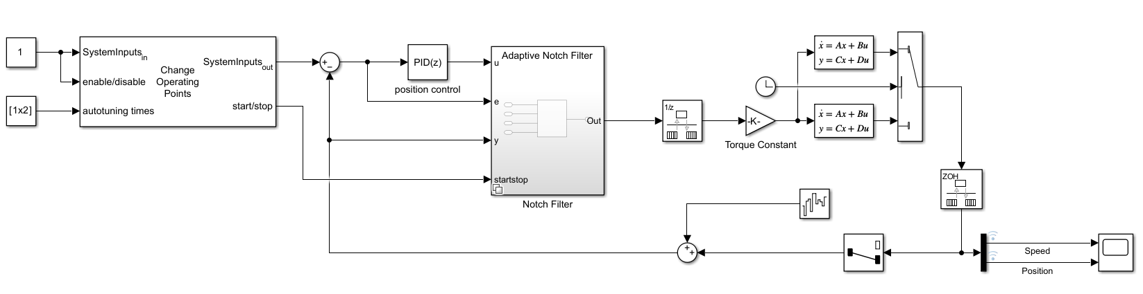
open_system(mdl)Model Overview
The model used in this example is composed of a linear state-space model, notch filter, PID controller, random noise, and a way to set the operating points. The state-space model is derived from a two inertia coupled system with spring and damper. For this example, the load inertia (J2) is changed during simulation to simulate a dispensing process. The PID controller is tuned to balance stability and response time and is set to control the load position of the system. Noise is added to the position output to simulate noise from sensors or other processes.
Plant Model
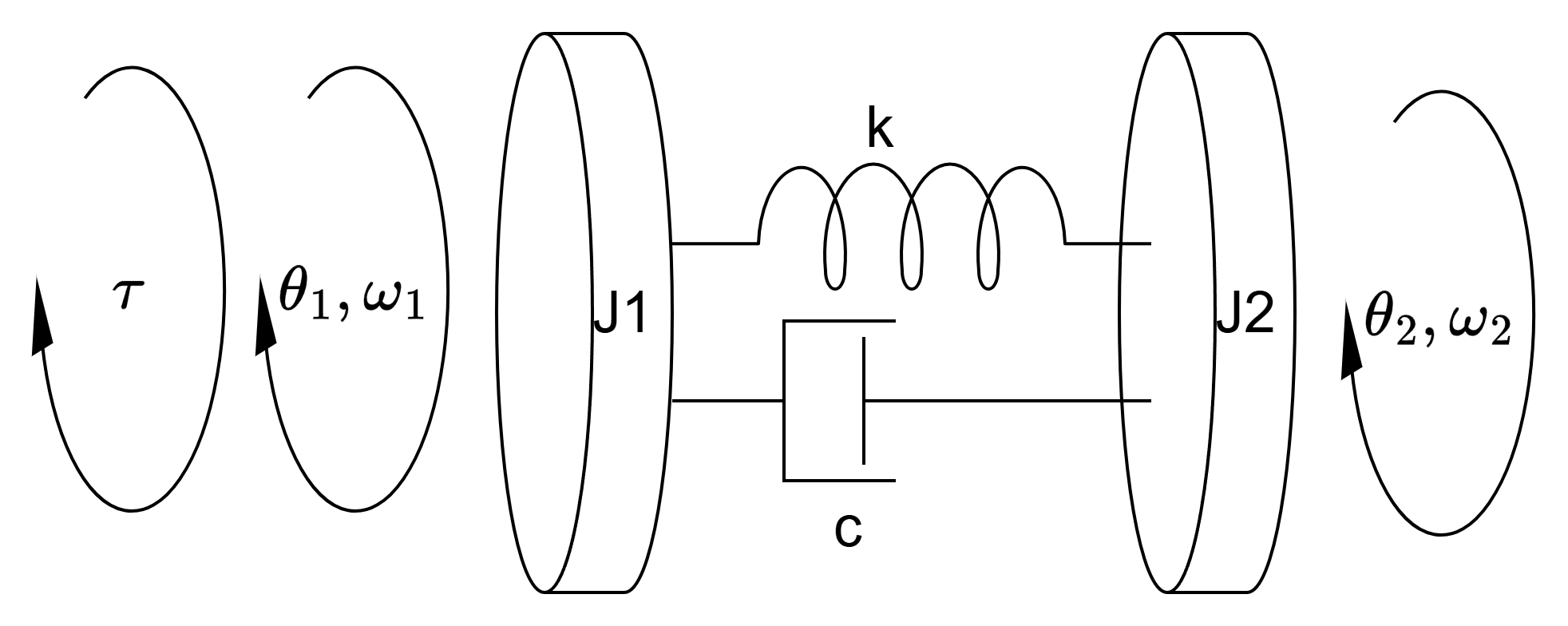
The plant model is based on a two inertia coupled system with a single spring and damper. For this example J1,k, and c remain constant over the course of the simulation but J2 is changed from 60 to 20 to simulate a loss of inertia commonly found in dispensing applications. The load position, , is used in the controller as this is typically measured using a position sensor. In addition, the speed of J1 is used in the results as this speed is also typically measured.
For use in simulation, the model is implemented using the Simulink® State-Space block which is configured to output the states mentioned previously.
Inertia Change
As mentioned in the previous section, the load inertia, J2, is changed during simulation to simulate a dispensing process losing mass. To achieve this two state-space models are used: one for the initial load inertia (J2 = 60) and a second after the load has been dispensed (J2 = 20). Plot the frequency response for the load position, , for these two state-space systems.
sys1 = ss(A,B,C(2,:),D(2,:));
sys2 = ss(A_2,B_2,C_2(2,:),D_2(2,:));
figure
bodeplot(sys1,sys2,{0.1 100})
legend("J2 = 60","J2 = 20")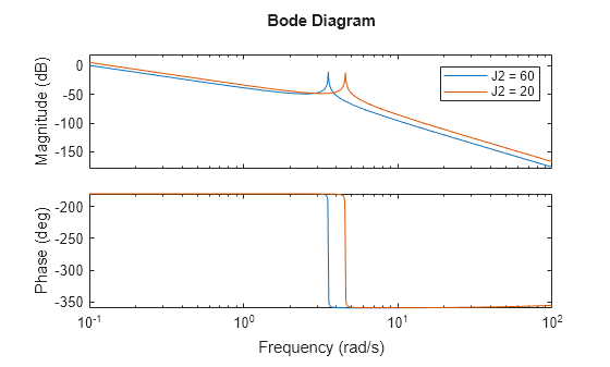
The resonance that is originally present at 3.54 rad/sec but changes to 4.56 rad/sec following the decrease in load inertia.
Compensating for Plant Resonance
The plant resonance that is present initially occurs around 3.54 rad/sec and results in oscillations in both speed and position. Because of this, it is desired to reduce these oscillations which can be done using a notch filter.
Using a Notch Filter to Remove Plant Resonance
You can use a notch filter to reduce the effect of the resonance seen by the control system. To properly set the parameters for the notch, the resonant frequency must first be determined using the following formula:
.
One formulation of the notch filter uses explicit settings for the depth and width of the notch. In this example, the values for the width and depth are 0.6 and 0.004, respectively. With all three parameters, you can determine the notch filter transfer function and apply to the state-space system.
notchDamp = 0.6;
notchGmin = 4e-3;
notchSys = tf([1 (2*notchGmin*notchDamp*notchFreq) (notchFreq^2)], [1 (2*notchDamp*notchFreq) (notchFreq^2)]);
Plot the bode diagram for the system both with and without the notch filter applied.
figure
bodeplot(sys1,sys1*notchSys,{0.1 100})
legend("Without notch","With notch")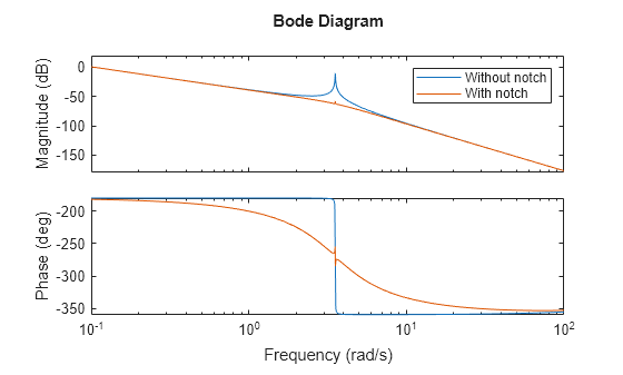
The inclusion of a notch filter placed at the resonant frequency improves the open-loop frequency response of the plant. However, if the notch filter is placed at the wrong frequency then the open-loop plant can be made worse. As shown in the figure below, the notch that is tuned to the frequency of the original plant (J2 = 60) is used on the plant with a lower load inertia (J2 = 20) (shown in red).
figure
bodeplot(sys2,sys2*notchSys,{0.1 100})
legend("Without notch", "Mismatched notch")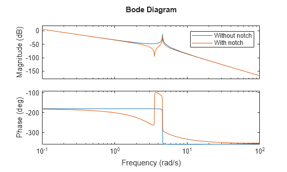
The overall plant response is made worse by using a notch that is set to the wrong frequency. There is now an anti-resonance at the original plants' resonant frequency (3.54 rad/sec) and the phase has been increased as well. From this result, it is clear that a single notch filter at one frequency will not be sufficient for a system whose resonance can change. One solution to this problem is to use a single notch filter that can adapt its frequency placement to handle a changing loading inertia.
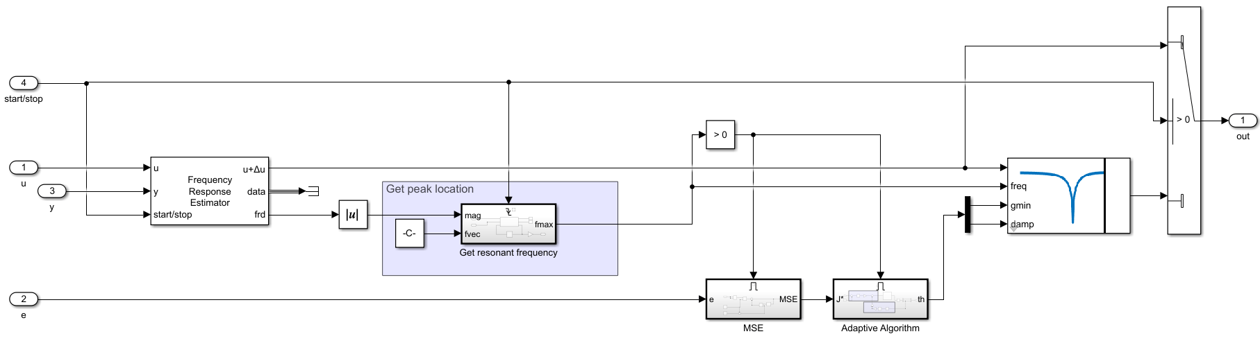
Adaptive Notch Filter (ANF) Overview
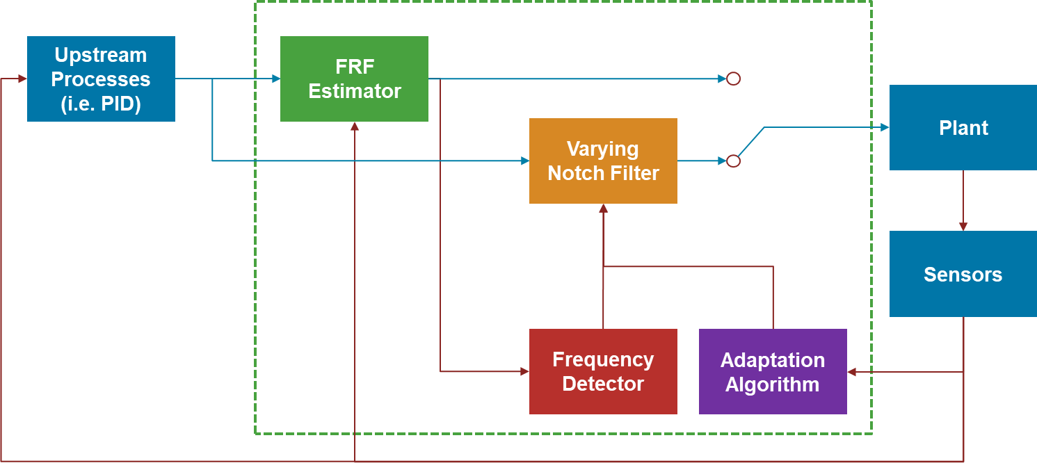
The above image shows a block diagram for the adaptive notch filter (ANF) used in this example. The ANF consists of four main parts:
Adaptation Algorithm
FRF Estimator
Frequency Detector
Notch Filter
The Adaptive Notch Filter block from Simulink® Control Design™ contains the Adaptation Algorithm the FRF Estimator, the Frequency Detector and the Varying Notch Filter. The FRF estimation and frequency detection portions are enabled when an external start/stop signal is used to trigger the estimation. During this time, the notch filter is bypassed and reenabled when a new frequency location for the notch is obtained.
The ANF will change its depth, width and frequency based on the ESC algorithm and the peak detector.
Using ANF to Reduce Effect of Plant Resonance for Changing Inertia
You can use this Adaptive Notch Filter block to handle a plant whose inertia (and thus resonance) changes. For this example, the system is commanded initially to a position of 1 then to position 2 at 1200 seconds. At 1600 seconds, the load inertia (J2) is changed from a value of 60 to 20 simulating a load being dispensed by a servo motor. At 2000 seconds the system is commanded to position 3 then finally to position 4 at 3000 seconds. Between positions 1 and 2 the plant resonance is estimated and then the adaptation algorithm for the adaptive notch filter is enabled. After the load has decreased the plant resonance is re-estimated and the location of the notch filter is updated.
This example simulates the model three times and the results of each simulation are compared:
Baseline with no notch filter
Single notch filter set at the
J2=60 resonant frequency (3.54 rad/sec)Adaptive notch filter
% Baseline simulation with no notch filter
sim(mdl)
baselineResults = logsout;

% Simulation with single notch filter tuned at 3.54 rad/sec
FilterType = 1;
sim(mdl)
staticNotchResults = logsout;

% Simulation with Adaptive Notch Filter
FilterType = 2;
sim(mdl)
adaptiveNotchResults = logsout;
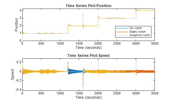
Compare the results from these three simulations. Plot the speed and position feedback over the entire 3500 second simulation.
figure
tiledlayout(2,1);

% Position
nexttile
plot(baselineResults{1}.Values)
hold on
plot(staticNotchResults{1}.Values)
plot(adaptiveNotchResults{1}.Values)
hold off
legend("No notch","Static notch", "Adaptive notch",Location="southeast")

% Speed
nexttile
plot(baselineResults{2}.Values)
hold on
plot(staticNotchResults{2}.Values)
plot(adaptiveNotchResults{2}.Values)
hold off
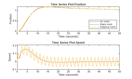
The overall response for the three cases differs significantly over the entire simulation. In order to examine each of the responses more closed, the plot can be zoomed in to each major event. The first plot below shows the initial transient from the initial state to position 1.
figure
tiledlayout(2,1);

% Position
nexttile
plot(baselineResults{1}.Values)
hold on
plot(staticNotchResults{1}.Values)
plot(adaptiveNotchResults{1}.Values)
hold off
xlim([0 50])
legend("No notch","Static notch","Adaptive notch",Location="southeast")

% Speed
nexttile
plot(baselineResults{2}.Values)
hold on
plot(staticNotchResults{2}.Values)
plot(adaptiveNotchResults{2}.Values)
hold off
xlim([0 50])
The response for the baseline result and the adaptive notch filter result are the same. This is because the ANF has not yet been tuned. However, the response with the static notch filter shows improved performance due to being tuned and set at the correct resonant frequency. The following plot below shows the transient from position 1 to position 2 after the notch filter has been tuned.
figure
tiledlayout(2,1);

% Position
nexttile
plot(baselineResults{1}.Values)
hold on
plot(staticNotchResults{1}.Values)
plot(adaptiveNotchResults{1}.Values)
hold off
xlim([1200 1250])
legend("No notch","Static notch","Adaptive notch",Location="southeast")

% Speed
nexttile
plot(baselineResults{2}.Values)
hold on
plot(staticNotchResults{2}.Values)
plot(adaptiveNotchResults{2}.Values)
hold off
xlim([1200 1250])
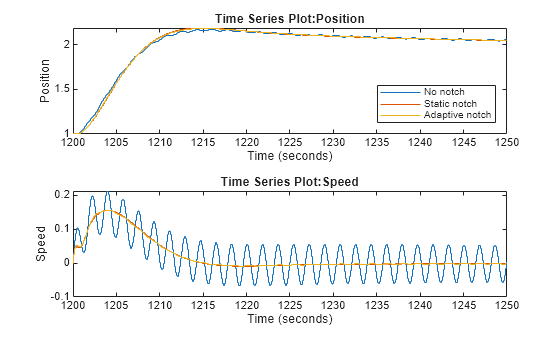
As shown in this plot, the adaptive notch filter response is comparable to the pretuned static notch filter because the ANF is enabled during this transient and its frequency placement was estimated using the frequency response estimator. The following plot below shows the transient from position 2 to position 3 after the load inertia has decreased from 60 to 20.
figure
tiledlayout(2,1);

% Position
nexttile
plot(baselineResults{1}.Values)
hold on
plot(staticNotchResults{1}.Values)
plot(adaptiveNotchResults{1}.Values)
hold off
xlim([2000 2050])
legend("No notch","Static notch","Adaptive notch",Location="southeast")

% Speed
nexttile
plot(baselineResults{2}.Values)
hold on
plot(staticNotchResults{2}.Values)
plot(adaptiveNotchResults{2}.Values)
hold off
xlim([2000 2050])
As shown in this plot, all three responses are poor but the simulation with no notch filter has the smallest oscillations. This is consistent with the above discussion showing that an improperly tuned notch filter causes the system performance to degrade compared to having no notch filter. The following plot shows the final transient from position 3 to position 4 after the adaptive notch filter's frequency has been re-estimated.
figure
tiledlayout(2,1);

% Position
nexttile
plot(baselineResults{1}.Values)
hold on
plot(staticNotchResults{1}.Values)
plot(adaptiveNotchResults{1}.Values)
hold off
xlim([3000 3050])
legend("No notch","Static notch","Adaptive notch",Location="southeast")

% Speed
nexttile
plot(baselineResults{2}.Values)
hold on
plot(staticNotchResults{2}.Values)
plot(adaptiveNotchResults{2}.Values)
hold off
xlim([3000 3050])
This plot shows that while the response of the system with no notch filter and a static notch filter have the same performance as before, the response with the adaptive notch filter is greatly improved due to its frequency placement changing to the new resonant frequency of 4.56 rad/sec.
Summary
In this example the resonance of a system is compensated for using a notch filter. The system experiences a change in load inertia causing the resonant frequency to move necessitating the need for either multiple notch filters or a single notch filter that adapts its frequency. The Adaptive Notch Filter block successfully changes its frequency placement following the change in load inertia and improves the overall system performance.