Extremum Seeking Control

Extremum seeking control (ESC) is a model-free, real-time adaptive control algorithm that is useful for adapting parameters to unknown system dynamics and unknown mappings from control parameters to an objective function. You can use extremum seeking to solve static optimization problems and to optimize parameters of dynamic systems.

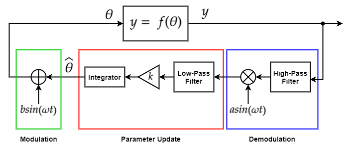
The extremum seeking algorithm uses the following stages to tune a parameter value.

Modulation — Perturb the value of the parameter being optimized using a low-amplitude sinusoidal signal.
System Response — The system being optimized reacts to the parameter perturbations. This reaction causes a corresponding change in the objective function value.
Demodulation — Multiply the objective function signal by a sinusoid with the same frequency as the modulation signal. This stage includes an optional high-pass filter to remove bias from the objective function signal.
Parameter Update — Update the parameter value by integrating the demodulated signal. The parameter value corresponds to the state of the integrator. This stage includes an optional low-pass filter to remove high-frequency noise from the demodulated signal.

Simulink^® Control Design™ software implements this algorithm using the Extremum Seeking Control block. For examples of extremum-seeking control, see:

Time Domain

Using the Extremum Seeking Control block, you can implement both continuous-time and discrete-time controllers. The ESC algorithm is the same in both cases. Changing the time-domain of the controller affects the time domain of the high-pass filters, low-pass filters, and integrators used in the tuning loops.

To generate hardware-deployable code for the Extremum Seeking Control block, use a discrete-time controller.

The following table shows the continuous-time and discrete-time transfer functions for the filters and integrators in the Extremum Seeking Control block.

Controller Element	Continuous-Time Transfer Function	Discrete-Time Transfer Function
High-pass filter	$\frac{s}{s + ω_{h}}$	$\frac{1 - z^{- 1}}{1 - ω_{h} z^{- 1}}$
Low-pass Filter	$\frac{1}{s + ω_{l}}$	$\frac{1}{1 - ω_{l} z^{- 1}}$
Integrator	$\frac{1}{s}$	Forward Euler: $\frac{T_{s}}{z - 1}$ Backward Euler: $\frac{T_{s} z}{z - 1}$ Trapezoidal: $\frac{T_{s}}{2} \frac{z + 1}{z - 1}$

Controller Element

Continuous-Time Transfer Function

Discrete-Time Transfer Function

High-pass filter

$\frac{s}{s + ω_{h}}$

$\frac{1 - z^{- 1}}{1 - ω_{h} z^{- 1}}$

Low-pass Filter

$\frac{1}{s + ω_{l}}$

$\frac{1}{1 - ω_{l} z^{- 1}}$

Integrator

$\frac{1}{s}$

Forward Euler:

$\frac{T_{s}}{z - 1}$

Backward Euler:

$\frac{T_{s} z}{z - 1}$

Trapezoidal:

$\frac{T_{s}}{2} \frac{z + 1}{z - 1}$

Here:

ω_l is the low-pass filter cutoff frequency.
ω_h is the high-pass filter cutoff frequency.
T_s is the sample time of the discrete-time controller learning rate.

Static Optimization

To demonstrate extremum seeking, consider the following static optimization problem.

Extremum seeking control diagram showing the modulation, demodulation, and parameter update stages.

Here:

$\hat{θ}$ is the estimated parameter value.
θ is the modulation signal
y = f(θ) is the function output being maximized, that is, the objective function.
ω is the forcing frequency of the modulation and demodulation signals.
b·sin(ωt) is the modulation signal.
a·sin(ωt) is the demodulation signal.
k is the learning rate.

The optimum parameter value, θ*, occurs at the maximum value of f(θ).

To optimize multiple parameters, you use a separate tuning loop for each parameter.

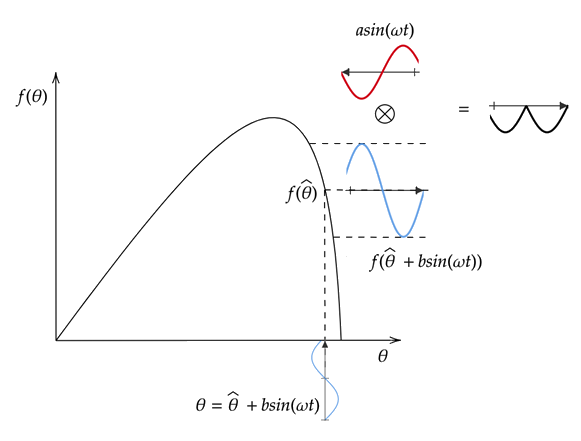
The following figure demonstrates extremum seeking for an increasing portion of the objective function curve. The modulated signal θ is the sum of the current estimated parameter and the modulation signal. Applying f(θ) produces a perturbed objective function with the same phase as the modulation signal. Multiplying the perturbed objective function by the demodulation signal produces a positive signal. Integrating this signal increases the value of θ, which moves it closer to the peak of the objective function.

Graph of an objective function with modulation and demodulation demonstrated on an increasing portion of the curve.

The following figure demonstrates extremum seeking for a decreasing portion of the objective function curve. In this case, applying f(θ) produces a perturbed objective function that is 180 degrees out of phase from the modulation signal. Multiplying by the demodulation signal produces a negative signal. Integrating this signal decreases the value of θ, which moves it closer to the peak of the objective function.

Graph of an objective function with modulation and demodulation demonstrated on a decreasing portion of the curve

The following figure demonstrates extremum seeking for a flat portion of the objective function curve, that is, a portion of the curve near the maximum. In this case, applying f(θ) produces a near-zero perturbed objective function. Multiplying by the demodulation signal and integrating this signal does not significantly change the value of θ, which is already near its optimum value θ*.

Graph of an objective function with modulation and demodulation demonstrated on a nearly flat portion of the curve

Dynamic System Optimization

Extremum seeking optimization of a dynamic system occurs in a similar fashion as static optimization. However, in this case, the parameter θ affects the output of a time-dependent dynamic system. The objective function to be maximized is computed from the system output. The following figure shows the general tuning loop for a dynamic system.

Extremum seeking for a time-dependent dynamic system.

Here:

$\dot{x} = f (x, α (x, θ))$ is the state function of the dynamic system.
z = h(x) is the output of the dynamic system.
y = g(z) is the objective function derived from the output of the dynamic system.
ϕ₁ is the phase of the demodulation signal.
ϕ₂ is the phase of the modulation signal.

ESC Design Guidelines

When designing an extremum-seeking controller, consider the following guidelines.

Ensure that the system dynamics are on the fastest time scale, the forcing frequencies are on the medium time scale, and the filter cutoff frequencies are on the slowest time scale.
Specify an amplitude for the demodulation signal that is much greater than the modulation signal amplitude (a ≫ b).
Select phase angles for the modulation and demodulation signals such that cos(ϕ₁ – ϕ₂) > 0.
When tuning multiple parameters, the forcing frequency for each tuning loop must be different.
Try designing your system without high-pass and low-pass filters. If the performance is not satisfactory, you can then consider adding one or both filters.

More About Extremum Seeking Control

For more information on extremum seeking control, play the video. This video is part of the Learning-Based Control video series.

In this video, I want to introduce an adaptive control method called Extremum Seeking Control. We're going to build up the algorithm in a way that I think will motivate each of the components, and hopefully highlight some of the overall benefits, and drawbacks of this method, I think Extremum Seeking Control is a really interesting and intuitive controller, so I hope you stick around for it. I'm Brian, and welcome to a MATLAB Tech Talk.

To begin, let's start with this generic system. There are signals u entering into the system and it produces some output, y. With feedback control, we're looking to design a controller that can use the outputs in some way to determine what the correct inputs are that, ultimately, get the system to behave the way we want. If we want to take an optimal approach to solving this problem, we need to set up some kind of cost function that we want to minimize, or an objective function that we want to maximize. And then find the parameters or the system inputs that do just that.

For example, a linear quadratic regulator is an optimal way to find the game matrix for full state feedback. We set up a quadratic cost function that takes into account system error and actuator effort. And then along with a model of the system dynamics, we can find the game matrix that perfectly blends effort and error together to produce the minimum overall cost.

Now, LQR requires a linear model of the system in order to do this optimization. Also, the optimization is done off-line and produces static gains and these aren't going to change over time, even if the system dynamics do. And the cost function has to be, by definition, quadratic. So the question is what if you don't have a model of your system, or if the system dynamics change over time and so a static gainsaid won't be sufficient, or if the cost or objective function that you're trying to optimize isn't quadratic. Then LQR isn't a good optimal solution.

For example, take an anti-lock braking system for your car, the input into this system is the amount of brake pressure to apply, and the output is the deceleration of the vehicle. How hard should we press the brakes to maximize deceleration? And the answer isn't obvious. If you apply too little brake pressure, you're not slowing down as fast as you can. And if you apply too much pressure, then the wheels will start to skid, which also reduces your braking effectiveness.

In fact, this interaction between the tire and the road is governed by a curve that looks something like this. So there's this perfect amount of brake pressure that will then cause the perfect amount of wheel slip that will maximize the braking force. And this is not a quadratic function. And also, this curve changes based on the road conditions, and the tire conditions. And not only is it changing, but to create a model of this system would require knowledge of the road surface, and the melting characteristics of rubber, and so much more. So because of these conditions, this is not a good candidate for LQR.

Now, there are a bunch of different ways to solve a problem like this, but I want to talk particularly about perturb and observe type algorithms. These algorithms don't require a system model, they don't require quadratic objective functions, and they can run real time and adapt to the changing system dynamics. And the basic algorithm works like this.

You start with an initial guess, in our case, that's a specific brake pressure. Then, we record the current objective value, which for us is the deceleration of the vehicle. Now, we perturb our best guess by stepping the input in one direction. Let's say we increase the brake pressure just a little bit. Now, we check to see if the objective increased or decreased to determine if that step was in the right direction.

For example, if the vehicle is decelerating more than it was previously, then we know that we've marched up the hill in the right direction and we keep that value. We then take another step, increasing the brake pressure some more and more and checking the result. Eventually, we'll reach the optimal braking pressure.

And now, at this point, we'll step past it and realize that the objective has decreased and therefore we've gone too far. Then, we step back in the other direction. And we have to keep stepping back and forth and back and forth around the maximum point, because a change in the environment or the system dynamics could move this maximum point around. And we always want to be probing for it and tracking it. And this is the basic idea of how we can find an optimal solution for a dynamic system without needing a model.

Now, there are some drawbacks to this very simple algorithm and one of which is that taking large steps will make it converge faster. But it's going to produce an average objective value that is lower than it could be, since you'd be jumping further away from the optimal value every step. Now, there are algorithms that try to estimate the gradient of the function and then use that to adjust the step size, so that when you're near the optimal point it doesn't take as large of steps.

And one version of this type of gradient estimating algorithm is Extremum Seeking Control, which is what we're going to talk about for the rest of this video. All right, so let's head over to Simulink and build this controller. I have here the plant that we wish to control and it takes a single input u, and it produces a single output. Now, in this case, the output is the objective that we're trying to maximize. However, in general this might not be the case.

We may take the outputs from the system and combine them with other signals in some way to generate an objective function. But to keep this simple, I've just wrapped it all up into this one system. So we're trying to find u that will maximize the output. And inside this function, you can see that it's just a really basic quadratic equation. And I'll show you what the result of this system looks like by ramping the input from 0 with a slope of 2 units per second.

Let me run this real quick and check out the scope. The yellow line here is the input ramping from 0. And you can see that right at u equals 10, the output reaches a maximum of 20. And this is the optimal condition for this particular system. And to relate this back to the breaking example, this is saying that a brake pressure of 10 units would produce the maximum deceleration. Anything more or less than this would result in a vehicle that takes longer to stop.

OK. So now, let's pretend that we don't actually know that an input of 10 is the optimal value and instead we have an initial guess of say five. We want our controller to automatically determine if five is too low, too high, or just right. And the way we're going to do that is to add a sine wave to this value. Basically, instead of feeding in a constant five, we're going to add a higher frequency ripple onto the signal that will perturb it slightly higher and lower.

And here I'm choosing a sine wave of 30 radiants per second with an amplitude of 0.3, but this is one of several places where the designer can tune the controller to their particular plant. Now, let's run this and check the scope. Again, the yellow line is the input signal with that sine wave ripple and the blue line is the system output.

Since five is lower than the optimal input, we'd expect that these two signals be in phase. That is when we increase five just a little bit, the objective also increases in phase with it. And if we change the input to 12, which is too high, we'd expect that the two signals then be out of phase. The trouble is, is that these two signals are hard to compare, in this state since they're offset from each other.

But luckily we don't necessarily care about the absolute value of these signals, we want to know how the change in the input signal creates a change in the output signal. The change in the input is easy to get, it's just the sine wave itself. But getting the change in the output is well, it's actually pretty easy also. We can do that by adding a high pass filter. I'm choosing one with a cutoff frequency of five radiants per second.

This will, essentially, block the low frequency information like the offset from 0 and pass the 30 radiant per second signal through without affecting it too much. And check it out. The offset has been removed by the high pass filter and we can now see clearly how the system output changes when we change the system input. And since these two signals are completely out of phase with each other, we know that we need to lower the input value to reach the maximum output.

So a value of 12 is too high. And if we change the input back to five, we can see that these two signals are now in phase with each other and, therefore, we know that the current input value of five is too low. But how do we get our controller to understand this kind of logic? Well, it turns out that we can just multiply the two signals together because if the two signals mostly have the same sign, like they have when they're in phase, then the product will be mostly positive.

And indeed, that is the case when the input is too low. You can see here that the signal is almost entirely positive. Well, let me first hide this yellow signal because it's cluttering up the scope. But now you can see that the signal is mostly above zero. And if we set our input to 12, you can see that the product is mostly below 0 since the two signals now have mostly opposite signs.

Finally, we can integrate this signal and then the summation will tend to rise when the input is too low and tend to decrease when the input is too high. And we can see here that the output from this integral is trending down, which indicates that 12 is too high and should be lowered. Now, not only does the summation increase when the input is too low and decrease if it's too high, but the speed with which it increases and decreases is proportional to the gradient, or the slope of the objective function.

To show you what I mean, let's set the input to a ramp and watch the summation as the input value sweeps through the optimal input. And how cool is this? The summation increases and decreases faster when we're further from the optimal value and then the steps get finer as we reach that goal. And then at the optimal value the sum stays constant and that's pretty awesome. And in this way, we can feedback this summation as our best guess of the input and then the system will ultimately converge on the optimal condition.

Well, ultimately, it will. This particular set up is taking its time to get there. But we have another tuning adjustment that we can make and that's to add gain to the summation, which will allow us to speed up and slow down convergence. Now, we have to be a little careful here because speeding it up too much will cause instability, but for us, this value looks OK. The input converges on 10, which produces the maximum output of 20.

And what's really cool about this controller is that it can adapt to changing plant dynamics. Well, as long as those dynamics are relatively slow compared to the convergence rate of the controller. The plant dynamics can't be faster than what the controller can converge to otherwise, it'll continuously lag behind the maximum value. Let me show you a quick example of the controller adapting to a changing plant by changing our plant equation to be a function of time.

Here I'm basically shifting the quadratic curve to the right as time increases, which means our controller needs to constantly increase the input value u, in order to maintain the maximum output value of 20. So let's run this. You can see that the output stays really close to the maximum value, but the input is constantly changing. It's tracking the value that creates the maximum output.

All right so these are the basic components that make up the Extremum Seeking Controller. And if you have Simulink Control Design, you can just pull in an Extremum Seeking Controller in to Simulink rather than write it all out yourself. And some of the benefits of using this block is that there is some error checking that is done for you, such as making sure that the frequencies between the modulating sine wave and the filters aren't stepping on each other.

Also, this block can handle multi-input and multi-output systems. And it exposes all of the configurable parameters in a single interface. But as you can see, the logic that it implements is exactly what we just walked through. Now, there is this extra low pass filter that can be used if there is high frequency measurement noise in your system, but I left it off since my example didn't have any measurement noise, but otherwise, exactly the same.

All right so hopefully you can see that we can use an algorithm like this to do something like track the ideal brake force that will stop a car in the shortest distance on an unknown surface. And if you're interested in seeing that in action, in the description there is a link to another video that shows how to use Extremum Seeking Control for anti-lock braking.

All right. Now, before we end this video, I want to really quickly talk about some of the drawbacks with this method so that you'll be more prepared to decide if it's right for your control problem. For one, this method will only converge on a local optimum. If your system has multiple optima, then you need to make sure that you initialize it such that it finds the global optimum. Also, even though it is a relatively straightforward controller, it is more complicated than a simple perturb and observe algorithm.

We have a lot of tuning parameters that we need to tweak to get the result that converges quickly and robustly on the optimal solution. And finally, we need a plant that responds quickly to input changes so that we can actually observe the perturbation, but a plant whose dynamics don't change too quickly over time so that the controller is capable of tracking the optimal point. But despite all of this, I hope that you can see that this is a pretty powerful controller if you're dealing with a system that's hard to model and changes over time.

And I think a good way to get more experience with Extremum Seeking Control is to just try it out yourself. And I've left links to examples and other documentation that should provide you with a good start. All right, so that's where I'm going to leave this video. If you don't want to miss any future Tech Talk videos, don't forget to subscribe to this channel. Also, if you want to check out my channel, Control System Lectures, I cover more controlled theory topics there as well. Thanks for watching, and I'll see you next time.

Video Player is loading.

Current Time 0:00

Duration 0:00

Loaded: 0%

Stream Type LIVE

Remaining Time 0:00

References

[1] Ariyur, Kartik B., and Miroslav Krstić. Real Time Optimization by Extremum Seeking Control. Hoboken, NJ: Wiley Interscience, 2003.