Model and Validate a System

Step 2 of 3 in Model-Based Design with Simulink

• 1
• 2
• 3

Model each component in the robot system to reflect its physical or functional behavior. Then, verify the model by simulating with test data. A Simulink^® model of a component is based on several starting points:

• An explicit mathematical relationship between the output and the input of a physical component — You can compute the outputs of the component from the inputs, directly or indirectly, through algebraic computations and integration of differential equations. For example, computation of the water level in a tank given the inflow rate is an explicit relationship. Each Simulink block executes based on the definition of the computations from its inputs to its outputs.

• An implicit mathematical relationship between model variables of a physical component — Because variables are interdependent, assigning an input and an output to the component is not straightforward. For example, the voltage at the positive (+) end of a motor connected in a circuit and the voltage at the negative (-) end have an implicit relationship. To model such a relationship in Simulink, you can use physical modeling tools such as Simscape™ or model these variables as part of a larger component that allows input/output definition. Sometimes, closer inspection of modeling goals and component definitions helps to define input/output relationships.

• Data obtained from an actual system — You have measured input/output data from the actual component, but a fully defined mathematical relationship does not exist. Many devices have unmodeled components that fit this description, for example, the heat dissipated by a television. You can use the System Identification Toolbox™ to define the input/output relationship for such a system.

• An explicit functional definition — You define the outputs of a functional component from the inputs through algebraic and logical computations, for example, the switching logic of a thermostat. You can model most functional relationships as Simulink blocks and subsystems.

This tutorial models physical and functional components with explicit input/output relationships. In this tutorial, you will:

1. Use the system equations to create a Simulink model.

2. Add and connect Simulink blocks in the Simulink Editor. Blocks represent coefficients and variables from the equations.

3. Build the model for each component separately. The most effective way to build a model of a system is to first consider components independently.

4. Start by building simple models using approximations of the system. Identify assumptions that can affect the accuracy of your model. Iteratively add detail until the level of complexity satisfies the modeling and accuracy requirements.

5. Validate components by supplying an input and observing the output.

Open System Layout

A big-picture view of the whole system layout is useful when modeling individual components. This model shows how the individual components are related to each other. Start by loading the system_layout model.

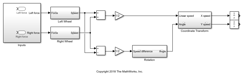
Model Physical Components

Describe the relationships between components, for example, data, energy, and force transfer. Use the system equations to build a graphical model of the robot system in Simulink.

Some questions to ask before you begin to model a component:

• What are the constants for each component? What values do not change unless you change them?

• What are the variables for each component? What values change over time?

• How many state variables does a component have?

Derive the equations for each component using scientific principles. Many system equations fall into three categories:

• For continuous systems, differential equations describe the rate of change for variables with the equations defined for all values of time. For example, a first-order differential equation gives the velocity of a car:

  $$\frac{dv(t)}{dt}=-\frac{b}{m}v(t)+u(t),$$

  where:

  • v(t) is the velocity of the car at time t.

  • b is the damping coefficient.

  • m is the mass of the car.

  • u(t) is the external force on the car at time t.

• For discrete systems, difference equations describe the rate of change for variables, but the equations are defined only at specific times. For example, this equation describes the control signal from a discrete proportional-derivative controller:

  $$u[n]=K_{p}e[n]+\text{}{K}_d\frac{\left(e[n]-e[n-1]\right)}{T_s},$$

  where:

  • u[n] is the control signal at the discrete time step n.

  • e[n] is the error at the discrete time step n.

  • e[n-1] is the error at the previous discrete time step n-1.

  • K_p is the proportional gain.

  • K_d is the derivative gain.

  • T_s is the sample time.

• Equations without derivatives are algebraic equations. For example, an algebraic equation gives the total current in a parallel circuit with two components:

  $$I_t=I_a+I_b,$$

  where:

  • I_t is the total current flowing through the circuit.

  • I_a is the current flowing through branch a of the parallel circuit.

  • I_b is the current flowing through branch b of the parallel circuit.

Model Linear Motion of Wheels

Two forces act on a wheel:

• Force applied by the motor — The force F acts in the direction of velocity change and is an input to the wheel subsystems.

• Drag force — The force F_drag acts against the direction of velocity change and is a function of velocity.

  $$F_{drag}=k_{drag}V\left|V\right|$$

Acceleration is proportional to the sum of these forces:

$$\begin{array}{c}(m/2)\dot{V}=F-F_{drag}\\ (m/2)\dot{V}=F-k_{drag}V\left|V\right|\\ \dot{V}=\frac{F-k_{drag}V\left|V\right|}{(m/2)},\end{array}$$

where k_drag is the drag coefficient and m is the mass of the robot. Each wheel carries half of this mass.

Build the wheel model:

1. In the system_layout model, double-click the subsystem named Right Wheel to display the empty subsystem.

2. To model velocity and acceleration, add an Integrator block. Leave the initial condition set to 0. The input of this block is the acceleration Vdot and the output is the velocity V.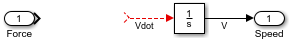

   

3. To model the drag force, add a MATLAB Function block from the User-Defined Functions library. The MATLAB Function block provides a quick way to implement mathematical expressions in your model. To edit the function, double-click the block to open the MATLAB Function Block Editor.

4. In the MATLAB Function Block Editor, enter the MATLAB^® code to calculate the drag force.

   function Fdrag=get_fdrag(V,k_drag)
   
   Fdrag=k_drag*V*abs(V);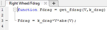

   

5. Define arguments for the MATLAB Function block. In the MATLAB Function Block Editor, click Edit Data . Click k_drag, and then set Type to Parameter Data.

6. Subtract the drag force from the motor force using the Subtract block. Complete the force-acceleration equation using a Gain block with the Gain parameter set to 1/(m/2).

7. To reverse the direction of the MATLAB Function block, select the block. Then, in the Simulink Toolstrip, on the Format tab, click Flip left-right . Connect the blocks.

   

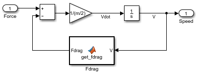
8. The dynamics of the two wheels are the same. Make a copy of the subsystem named Right Wheel that you just created and paste it in the subsystem named Left Wheel.

To view the parent model, click Up To Parent .

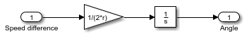
Model Rotational Motion of Wheels

When the two wheels turn in opposite directions, they move in a circle of radius r, causing rotational motion of the robot. When the wheels turn in the same direction, there is no rotation. Assuming that the wheel velocities are always equal in magnitude, you can model rotational motion as dependent on the difference of the two wheel velocities V_R and V_L:

$$\dot{\theta }=\frac{V_R-V_L}{2r}$$

Build the rotation dynamics model:

1. In the top level of the system_layout model, double-click the subsystem named Rotation to display the empty subsystem. Delete the connection between the Inport and the Outport blocks.

2. To model angular speed and position, add an Integrator block. Leave the initial condition set to 0. The output of this block is the rotational position $$\theta$$ and the input is the angular speed $$\dot{\theta }$$.

3. Compute angular speed from tangential speed. Add a Gain block and set the Gain parameter for the block to 1/(2*r).

4. Connect the blocks.

   

To view the parent model, click Up To Parent .

Model Functional Components

Describe the function from the input of a function to its output. This description can include algebraic equations and logical constructs, which you can use to build a graphical model of the system in Simulink.

Model Coordinate Transformation

The velocity of the robot in the x and y coordinates, V_X and V_Y, is related to the linear speed V_N and the angle $$\theta$$:

$$\begin{array}{l}{V}_X=V_N\cos \left(\theta \right)\\ V_Y=V_N\sin \left(\theta \right)\end{array}$$

Build the coordinate transformation model:

1. In the top level of the system_layout model, double-click the subsystem named Coordinate Transform to display the empty subsystem.

2. To model trigonometric functions, add a SinCos block from the Math Operations library.

3. To model multiplication, add two Product blocks from the Math Operations library.

4. Connect the blocks.

   

To view the parent model, click Up To Parent .

Set Model Parameters

You can determine appropriate values for parameters in your model using several sources, including:

• Written specifications such as standard property tables or manufacturer data sheets

• Direct measurements on an existing system

• Estimations using system input/output

The system_layout model uses these parameters.

Parameter	Symbol	Value
Mass	m	2.5 kg
Rolling resistance	k_drag	30 Ns2/m
Robot radius	r	0.15 m

A Simulink model can access parameter values defined using variables in the MATLAB workspace. Define these variables by entering the commands in the MATLAB Command Window.

m = 2.5;
k_drag = 30;
r = 0.15;

Validate Components

Validate components by supplying an input and observing the output. Even such a simple validation can point out immediate ways to improve the model. This example validates these behaviors:

• When a force is applied continuously to a wheel, the velocity increases until it reaches a steady-state velocity.

• When the wheels turn in opposite directions, the rotation angle increases at a constant rate.

This example uses Outport blocks to log output data to the workspace and the Simulation Data Inspector. For more information about logging data and other logging techniques, see Save Simulation Data.

Validate Wheel Component

Create and run a test model for the wheel component:

1. Create a new model. In the Simulation tab, click New . Copy the Subsystem block named Right Wheel into the new model.

2. To create a test input, add a Step block from the Sources library and connect it to the input of the subsystem named Right Wheel. Leave the Step time parameter set to 1.

3. To log output, connect the subsystem to an Outport block.

   

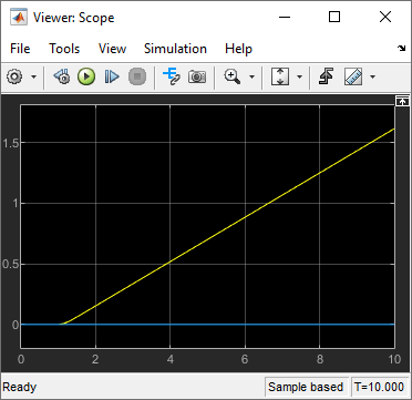
4. Simulate the model. In the Simulation tab, click Run .

5. To view the results in the Simulation Data Inspector, click Data Inspector . To plot the data, select the check box next to the Speed:1 signal.

   

The simulation results show that the model exhibits the general expected behavior. No motion occurs until force is applied at the step time. When force is applied, the speed starts to increase and then settles at a constant when the applied force and the drag force reach an equilibrium. In addition to validation, this simulation also shows the maximum speed of the wheel for the given force.

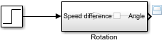
Validate Rotation Component

Create and run a test model for the rotation model:

1. To create a new model, click New . Copy the subsystem block named Rotation into the new model.

2. To create a test input in the new model, add a Step block from the Sources library. Leave the Step time parameter set to 1. Connect the output of the Step block to the input of the subsystem named Rotation. This input represents the difference of the wheel velocities when the wheels rotate in opposite directions.

3. To log output, connect the subsystem to an Outport block.

   

4. Simulate the model. In the Simulation tab, click Run .

5. To view the results in the Simulation Data Inspector, click Data Inspector . To plot the data, select the check box next to the Angle:1 signal.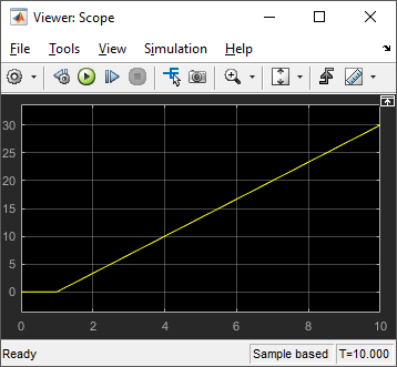

   

This simulation shows that the angle increases steadily when the wheels are turning with the same speed in opposite directions. You can improve the model to make the angle output easier to interpret. For example, you can:

• Convert the output signal units from radians to degrees by adding a Gain block with a gain of 180/pi.

• Display the output value in cycles of 360 degrees by adding a Math Function block with function mod.

MATLAB trigonometric functions take inputs in radians.

Validate Model

After you validate individual components, you can perform a similar validation on the complete model. This example validates these behaviors:

• When the same force is applied to both wheels in the same direction, the robot moves in a line.

• When the same force is applied to both wheels in opposite directions, the robot rotates in place.

Test Wheels Spinning in Same Direction

When the wheels are both spinning in the same direction, the robot should move in a line.

1. In the system_layout model, double-click the subsystem named Inputs to display the empty subsystem.

2. Create a test input by adding a Step block. Leave the Step time parameter set to 1. Connect the Step block output to both Outport blocks.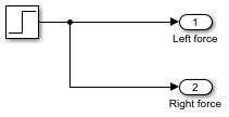

   

3. At the top level of the model, connect both Integrator blocks to Outport blocks to log the data. Label the signals X position and Y position.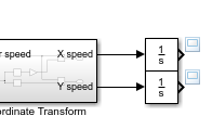

   

4. Simulate the model.

5. In the Simulation Data Inspector, select the X position and Y position signals to view the results.

Since the angle is zero and does not change, the vehicle moves only in the x direction, as expected.

Test Wheels Spinning in Opposite Directions

When the wheels spin in opposite directions, the robot should rotate in place.

1. Double-click the subsystem named Inputs. To reverse the direction for the left wheel, add a Gain block between the source and the second output and set the Gain parameter to -1.

   

2. Mark the angle output for signal logging. Right-click the output signal from the subsystem block named Rotation and click Log Selected Signals.

3. Simulate the model.

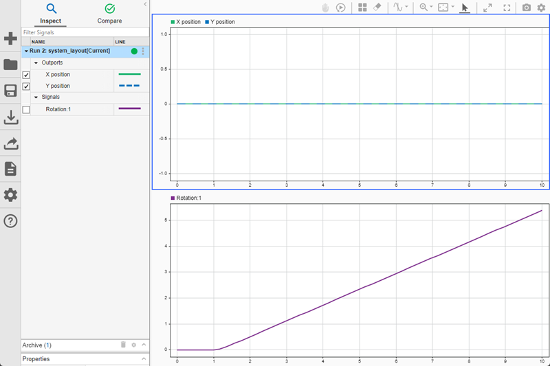
4. View the signals in the Simulation Data Inspector using two vertically aligned subplots. Click Visualizations and Layouts . Then, under Basic Layouts, choose the 2× 1 layout. In the upper subplot, plot the X position and Y position signals. In the lower subplot, plot the Rotation:1 signal.

The upper subplot shows that no motion occurs in the X-Y plane. The lower subplot shows steady angular motion.

You can use this final model to explore different scenarios by changing the input:

• Observe what happens when you set the initial angle to a value other than zero.

• Note how long it takes for the motion to stop when the force drops to zero.

• Increase the weight of the robot. Observe what happens when the robot is heavier.

• See how the robot moves on a smoother surface with a smaller drag coefficient.