Design a System in Simulink

Step 3 of 3 in Model-Based Design with Simulink

• 1
• 2
• 3

Model-Based Design centers on models of physical components and systems as a basis for design, testing, and implementation activities. This tutorial shows you how to add a designed component to an existing system model by adding an alert system to a model of a flat robot.

Open System Model

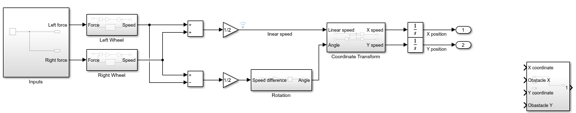
This model is a flat robot that can move or rotate with the help of two wheels, similar to a home vacuuming robot.

Identify Designed Components and Design Goals

Specifying the design objective is a critical first step to the design task. Even a simple system can have multiple and even competing design goals. Consider these goals for the example model:

• Design a controller that varies the force input so that the wheels turn at a desired speed.

• Design inputs that make the device move in a predetermined path.

• Design a sensor and controller so that the device follows a line.

• Design a planning algorithm so that the device reaches a certain point using the shortest path possible while avoiding obstacles.

• Design a sensor and algorithm so that the device moves over a certain area while avoiding obstacles.

This tutorial shows you how to design an alert system. Use the existing model to determine the parameters needed for a sensor that measures the distance from an obstacle. This example assumes a perfect sensor that measures the distance accurately. An alert system samples these measurements at fixed intervals to keep the output within 0.05 m of the measurement, triggering an alert in time for the robot to stop before a hitting the obstacle.

Analyze System Behavior Using Simulation

The design of the new component requires analyzing the linear motion of the robot to determine:

• How far the robot can travel at the top speed when power to the wheels is cut

• The top speed of the robot

Simulate the model with a force input signal that starts motion, waits until the robot reaches a steady velocity, and then sets the force to zero:

1. In the model, double-click the subsystem named Inputs.

2. Delete the existing step input and add a Pulse Generator block.

3. Set these parameters for the Pulse Generator block:

   • Amplitude: 1

   • Period: 20

   • Pulse Width: 15

   These parameter values help the robot to reach top speed. You can change parameters to see how different values affect the movement of the robot.

4. Simulate the model for 20 seconds.

5. Analyze the simulation results. To open the Simulation Data Inspector, click Data Inspector. This model logs data for the linear speed, X position, and Y position signals.

   Change the subplot layout to view all three signals. Click the Visualizations and Layouts button . Then, under Basics, choose the split bottom layout .

   • In the top subplot, plot the linear speed signal.

   • In the bottom-left subplot, plot the X position signal.

   • In the bottom-right subplot, plot the Y position signal.

   

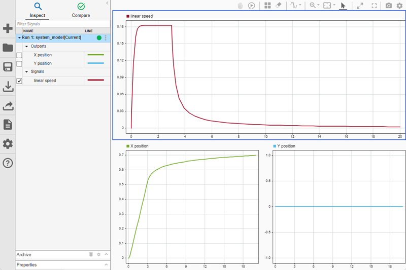
   The upper subplot shows that the speed of the robot rapidly decreases after the pulse that represents the input force drops to 0 at a simulation time of 3 seconds. The speed asymptotically approaches 0 but never reaches 0. Accurate modeling for low-speed dynamics without external forces requires a more complex representation of the system. However, this approximate representation of the system is sufficient for the purpose of the example.

   The lower subplots shows the x and y position of the robot over the course of the simulation. The robot does not move in the y direction. In the x direction, at the start of the simulation, the position changes rapidly. At about a simulation time of 3 seconds, the position changes more slowly as the speed of the robot decreases.

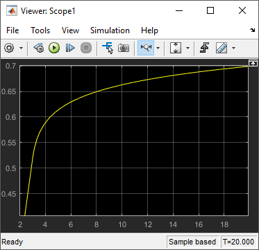
You can zoom and pan to find the final position of the robot. Click the Zoom in button , and then click and drag to zoom in on the bottom-left subplot that shows the robot position. At time 3 seconds, the position of the robot is approximately 0.55 m. At the end of the simulation, the position of the robot is approximately 0.7 m. Because the speed of the robot is close to zero at the end of the simulation, the results show that the robot moves less than 0.16 m after the external force drops to zero.

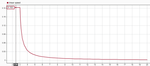
You can use cursors to find the top speed. Click the Show/hide data cursors button . Position the cursor in the region where the velocity curve is flat. The data cursor label shows that the top speed of the robot is 0.183 m/s. To calculate how long the robot takes to travel 0.05 m, divide 0.05 m by 0.183 m/s to get the result of 0.27 sec.

Design Components and Verify Design

Sensor design consists of these components:

• Measurement of the distance between the robot and the obstacle — This example assumes that the measurement is perfect.

• The time interval between each distance measurement the alert system makes — To keep the measurement error below 0.05 m, the sampling interval must be less than 0.27 sec. Use 0.25 sec.

• The distance at which the sensor produces an alert — Analysis shows that slow down must start by the time the robot is approximately 0.16 m from the obstacle. The actual alert distance must also take the error from discrete measurements, 0.05 m, into account.

Add Designed Component

Build the sensor:

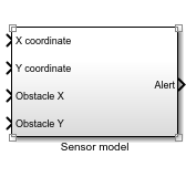
1. Create a subsystem with four input ports and one output port. The subsystem receives inputs for the x- and y-coordinates of the robot and for the x- and y-coordinates of the obstacle. The alert signal produced by the sensor connects to the output port.

   

2. Construct the distance measurement subsystem. In the subsystem named Sensor model, use the Subtract block, the Math Function block with the function magnitude^2, the Sum block, and the Sqrt block to implement the distance calculation. Notice that within the subsystem, the arrangement of the input ports does not need to match the arrangement of the ports on the Subsystem block interface.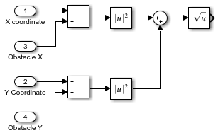

   

3. To model the sampling, add a Zero-Order Hold block to the subsystem from the Discrete library and set the Sample time parameter for the block to 0.25.

4. Connect the result of the distance calculation to the input of the Zero-Order Hold block.

5. To model the alert logic, add a Compare to Constant block from the Logic and Bit Operations library and set these block parameters:

   • Operator: <=

   • Constant Value: 0.21

   • Output data type: boolean

   With these parameter values, the block output value is 1 when the input value, which indicates the distance between the robot and the obstacle, is less than or equal to 0.21.

6. Connect the output of the Zero-Order Hold block to the input of the Compare to Constant block.

7. Finally, connect the output of the Compare to Constant block to the Outport block named Alert.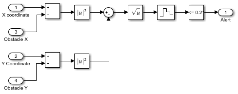

   

Verify Design

Test the design with an obstacle location of X = 0.65, Y = 0 using Constant blocks as inputs to the Sensor model subsystem. This test verifies design functionality in the X direction. You can create similar tests for different paths. This model only generates an alert and does not control the robot.

1. Set the obstacle location. Add two Constant blocks from the Sources library set the constant values to 0.65 and 0. Connect the position outputs of the robot to the inputs of the sensor.

2. Connect an Outport block to the Sensor model subsystem to log the data.

3. Mark the X position and Y position signals for signal logging. Select both signals. On the Simulation tab, click Log Signals.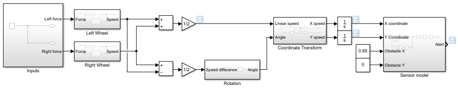

   

4. Simulate the model.

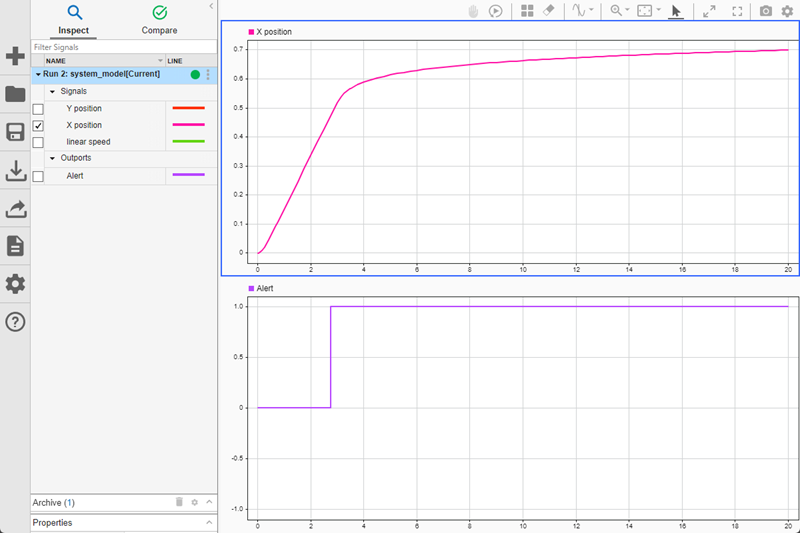
In the Simulation Data Inspector, click the Visualizations and Layouts button to change the plot layout to a 2×1 layout. In the upper subplot, plot the X position signal. In the lower subplot, plot the Alert signal.

The plot of the robot position looks the same as in the previous run. The plot of the alert signal shows that the alert signal value becomes 1 when the robot comes within 0.21 m of the obstacle location, satisfying the design requirement for this component.

For real-world systems with complex components and formal requirements, the Simulink^® product family includes additional tools to refine and automate the design process. Requirements Toolbox™ provide tools to formally define requirements and link them to model components. Simulink Control Design™ can facilitate the design if you want to build a controller for this robot. Simulink Verification and Validation™ products establish a formal framework for testing components and systems.