Automated Labeling of Time-Frequency Regions for AI-Based Spectrum Sensing Applications
The time-frequency representation of a signal often contains rich information that can be utilized for various tasks, such as signal classification and detection. Labeled time-frequency maps, like spectrograms, can be used to train segmentation and detection models to identify RF waveforms in spectrum sensing applications. However, manually labeling and maintaining a time-frequency labeling data set is an extremely tedious and time-consuming process. By incorporating rule-based methods or leveraging unsupervised learning techniques, you can partially automate this workflow, significantly aiding manual labeling efforts and reducing labor costs.
This example divides the automatic labeling process into two parts:
Automatic Region-of-Interest (ROI) Localization: Determine the boundaries of the regions containing signals.
Automatic ROI Clustering: Cluster the signal regions into multiple groups.
The example demonstrates how unsupervised learning methods can automate the localization and clustering to obtain clustered bounding boxes for regions in the time-frequency spectrum that may contain meaningful signals. The clustering result serves as an excellent starting point for further manual annotation, greatly reducing the cost of manual labeling.
Loading Data
This example uses a data set [1] comprising 20,000 spectrograms generated using a Rohde and Schwarz® SMBV100B vector signal generator to create RF frames consisting of Wi-Fi® and Bluetooth® signals, which are then recorded by a USRP N310 SDR. The frames are randomly arranged with channel models applied to simulate realistic RF environments, including frame collisions, where multiple RF signals overlap in time and frequency, potentially causing interference and making signal separation and decoding more challenging. The final composite signals are converted into labeled spectrogram images, providing a diverse dataset for deep learning-based RF frame detection.
Specifically, the dataset consists of 20,000 spectrograms distributed in frames, as follows:
- Approximately 362,780 Wi-Fi® frames
- 21,340 frames of Bluetooth® Low Energy (BLE) 1 MHz
- 21,340 BLE 2 MHz frames
- 21,340 Bluetooth® frames
- 77,600 collisions between different frames
For convenience, this example uses one observation sampled at 25 MHz to demonstrate the workflow steps. Start by reading the complex-valued time-domain signal and plotting its spectrogram magnitude.
unzip("TFLabeling.zip",pwd)
datafolder = "TFLabeling";
filename = "frame_138769090459325560_bw_25E+6.mat";

filepath = fullfile(datafolder,filename);
file = load(filepath);
sig = file.complex_array';
fs = 25e6;
win = hann(256);

figure(Position=[0 0 1000 300])
[S,f,t] = stft(sig,fs,FrequencyRange="centered",Window=win);
Smag = abs(S);
stft(sig,fs,FrequencyRange="centered",Window=win)
set(gca,YDir="reverse")
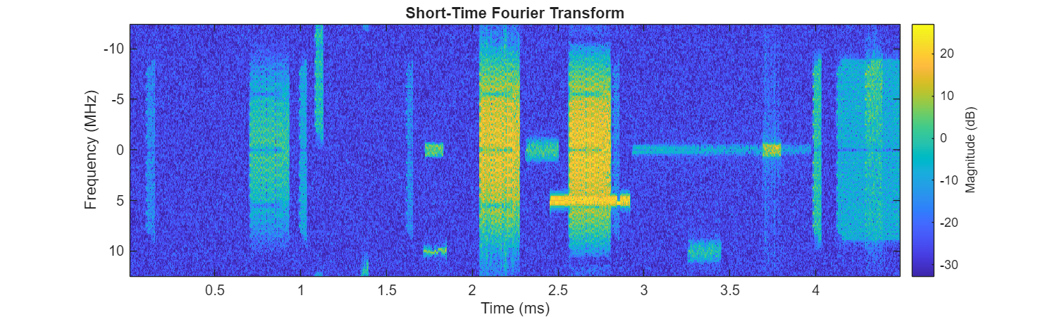
The spectrogram clearly shows the presence of frames that correspond to Wi-Fi®, BLE, and Bluetooth® bands. Different signals have different time-frequency signatures that a communications expert can label manually. However, the manual delimitation of the signal regions and labels can become costly for a large dataset like the one at hand. Having an automated process to label the time-frequency images can be of great value.
Localization of ROIs
The first step is to locate the regions of interest by identifying the boundaries of each signal in the time-frequency domain, i.e., locate the regions of interest. This task is not trivial, especially when processing large dataset of collected signals that include multiple signal intensities. Manual boundary selection is time-consuming, labor-intensive, and prone to human errors. It is therefore important to develop methods to automate annotation or to assist in manual annotation.
Localization Using Locally Adaptive Grayscale Threshold
A typical way to get started is to consider the spectrogram as a grayscale image. Using a locally adaptive threshold enables you to distinguish regions containing signals (foreground) from those without signals (background).
Use the helperFindSpecROI function with the Method parameter specified as "adaptthresh". This method uses the Image Processing Toolbox adaptthresh function. The helper function performs these steps:
Preprocess the image using
imdilateto smooth the spectrogram to some extent.Use
adaptthreshto segment the preprocessed spectrogram.Extract the segmentation results, collect the bounding boxes, and save and organize them into a table format.
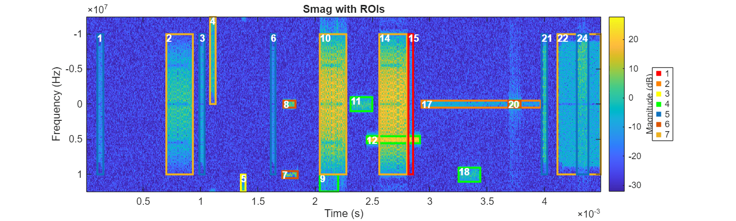
ROITableThresh = helperFindSpecROI(Smag,f,t,Method="Adaptthresh");
figure(Position=[0 0 1000 300])
helperPlotROIs(Smag,f,t,ROITableThresh)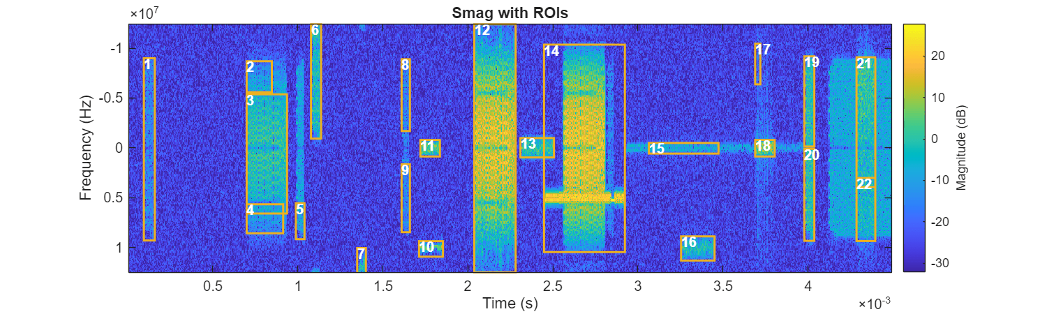
The resulting table contains this information:
Index: Region number.BoundingBox: Position and size of the smallest rectangle that can contain the region, formatted as a 1-by-4 vector[xmin ymin width height]in pixels. For example, a 2-D bounding box with values[5.5 8.5 11 14]indicates that the (x, y) coordinate of the top-left corner of the box is (5.5, 8.5), the horizontal width of the box is 11 pixels, and the vertical height of the box is 14 pixels.BoundingBoxTF: A similar bounding box vector but in time-frequency units, where the y-axis unit is MHz and the x-axis unit is ms.
disp(ROITableThresh)
    Index                BoundingBox                                      BoundingBoxTF
    _____    ____________________________________    _______________________________________________________

      1        35.5      35.5        25       188     9.472e-05    -8.9844e+06     6.3964e-05     1.8288e+07
      2       271.5      38.5        58        32    0.00069888    -8.6914e+06      0.0001484     3.1128e+06
      3       271.5      72.5        93       123    0.00069888    -5.3711e+06     0.00023794     1.1965e+07
      4       271.5     185.5        84        30    0.00069888     5.6641e+06     0.00021492     2.9182e+06
      5       384.5     184.5        20        37    0.00098816     5.5664e+06     5.1171e-05     3.5992e+06
      6       419.5       0.5        23       118     0.0010778    -1.2402e+07     5.8846e-05     1.1478e+07
      7       525.5     230.5        20        26     0.0013491     1.0059e+07     5.1171e-05     2.5291e+06
      8       627.5      36.5        19        74     0.0016102    -8.8867e+06     4.8612e-05     7.1983e+06
      9       627.5     144.5        19        70     0.0016102     1.6602e+06     4.8612e-05     6.8092e+06
     10       667.5     223.5        55        16     0.0017126      9.375e+06     0.00014072     1.5564e+06
     11       670.5     119.5        45        17     0.0017203    -7.8125e+05     0.00011513     1.6537e+06
     12       794.5       0.5        95       256     0.0020378    -1.2402e+07     0.00024306     2.4902e+07
     13       900.5     117.5        77        20     0.0023091    -9.7656e+05     0.00019701     1.9455e+06
     14       954.5      21.5       186       214     0.0024474    -1.0352e+07     0.00047589     2.0817e+07
     15      1195.5     122.5       160        11     0.0030643    -4.8828e+05     0.00040937       1.07e+06
     16      1269.5     218.5        77        25     0.0032538     8.8867e+06     0.00019701     2.4319e+06
     17      1439.5      20.5        12        42      0.003689    -1.0449e+07     3.0702e-05     4.0855e+06
     18      1439.5     119.5        45        17      0.003689    -7.8125e+05     0.00011513     1.6537e+06
     19      1552.5      33.5        23        93     0.0039782    -9.1797e+06     5.8846e-05     9.0466e+06
     20      1552.5     128.5        23        95     0.0039782          97656     5.8846e-05     9.2411e+06
     21      1672.5      34.5        43       134     0.0042854     -9.082e+06     0.00011002     1.3035e+07
     22      1672.5     158.5        43        65     0.0042854     3.0273e+06     0.00011002     6.3229e+06
Filtering ROIs Based on Metrics
This process has successfully labeled all regions containing signals with bounding boxes. However, some bounding boxes are false alarms that do not contain specific signals. You can apply criteria such as magnitude, size, or frequency range to filter these out these unwanted bounding boxes.
The annotated spectrogram in the previous step shows that points within regions containing actual signals usually have magnitudes above a certain threshold. Therefore, set the threshold as the median magnitude of all the points in the region. Regions below the threshold are filtered out.
Use the helperExtractFeatures function to extract the features and add them to the table. Set the feature name MedianMag to true to include this feature. The returned table includes the newly computed feature.
ROITableThreshFeature = helperExtractFeatures(ROITableThresh, ...
    TFMap=Smag, ...
    MedianMag=true);
disp(ROITableThreshFeature)
    Index                BoundingBox                                      BoundingBoxTF                         MedianMag
    _____    ____________________________________    _______________________________________________________    _________

      1        35.5      35.5        25       188     9.472e-05    -8.9844e+06     6.3964e-05     1.8288e+07     0.11789
      2       271.5      38.5        58        32    0.00069888    -8.6914e+06      0.0001484     3.1128e+06     0.23098
      3       271.5      72.5        93       123    0.00069888    -5.3711e+06     0.00023794     1.1965e+07     0.67904
      4       271.5     185.5        84        30    0.00069888     5.6641e+06     0.00021492     2.9182e+06     0.23917
      5       384.5     184.5        20        37    0.00098816     5.5664e+06     5.1171e-05     3.5992e+06     0.19923
      6       419.5       0.5        23       118     0.0010778    -1.2402e+07     5.8846e-05     1.1478e+07     0.46177
      7       525.5     230.5        20        26     0.0013491     1.0059e+07     5.1171e-05     2.5291e+06     0.15575
      8       627.5      36.5        19        74     0.0016102    -8.8867e+06     4.8612e-05     7.1983e+06     0.12104
      9       627.5     144.5        19        70     0.0016102     1.6602e+06     4.8612e-05     6.8092e+06     0.13195
     10       667.5     223.5        55        16     0.0017126      9.375e+06     0.00014072     1.5564e+06     0.18154
     11       670.5     119.5        45        17     0.0017203    -7.8125e+05     0.00011513     1.6537e+06     0.79304
     12       794.5       0.5        95       256     0.0020378    -1.2402e+07     0.00024306     2.4902e+07      1.5027
     13       900.5     117.5        77        20     0.0023091    -9.7656e+05     0.00019701     1.9455e+06     0.63091
     14       954.5      21.5       186       214     0.0024474    -1.0352e+07     0.00047589     2.0817e+07     0.36156
     15      1195.5     122.5       160        11     0.0030643    -4.8828e+05     0.00040937       1.07e+06     0.27532
     16      1269.5     218.5        77        25     0.0032538     8.8867e+06     0.00019701     2.4319e+06      0.3399
     17      1439.5      20.5        12        42      0.003689    -1.0449e+07     3.0702e-05     4.0855e+06     0.08331
     18      1439.5     119.5        45        17      0.003689    -7.8125e+05     0.00011513     1.6537e+06       1.359
     19      1552.5      33.5        23        93     0.0039782    -9.1797e+06     5.8846e-05     9.0466e+06     0.55955
     20      1552.5     128.5        23        95     0.0039782          97656     5.8846e-05     9.2411e+06     0.56903
     21      1672.5      34.5        43       134     0.0042854     -9.082e+06     0.00011002     1.3035e+07     0.74048
     22      1672.5     158.5        43        65     0.0042854     3.0273e+06     0.00011002     6.3229e+06     0.53959
Try different thresholds to remove unwanted areas.
threshold =0.1; selectedidx = ROITableThreshFeature{:,"MedianMag"} > threshold; ROITableThreshSelect = ROITableThreshFeature(selectedidx,:); figure(Position=[0 0 1000 300]) helperPlotROIs(Smag,f,t,ROITableThreshSelect)

The results are more accurate after applying the filtering operation. However, there are still some issues. For example, regions 5 and 15 do not fully cover the complete signal boundaries. Other signals, like in region 14, have regions that are larger than their true time-frequency content. These issues can be avoided by applying more preprocessing to the spectrogram and adjusting the parameters of adaptive thresholding. However, this may require numerous trials and significant manual effort.
Localization of ROIs Using the Segment Anything Model (SAM)
There are some other methods available for ROI localization. Deep learning models have greatly succeeded in image segmentation and object recognition, with many demonstrating significant generalization and transfer learning abilities. Next, use the pre-trained Segment Anything Model (SAM) [2] for effective region localization.
SAM is a model that was trained on the Segment Anything 1 Billion (SA-1B) dataset. Although SAM was not specifically trained for spectrograms, SAM has strong generalization capabilities and can effectively segment spectrograms with minimal parameter fine tuning. For more information about SAM, see Get Started with Segment Anything Model for Image Segmentation (Image Processing Toolbox).
Use the helperFindSpecROI function with the Method parameter specified as "SAM". It performs the following steps:
Preprocess the image using
imdilateto smooth the spectrogram.Use SAM to segment the preprocessed spectrogram.
Extract the segmentation results from SAM, collect the bounding boxes, and save and organize them into a table format.
Segmentation can be time-consuming. To save time, you can skip this step by loading pre-computed results instead.
segmentNow =false; if segmentNow ROITableSAM = helperFindSpecROI(Smag,f,t,Method="SAM"); %#ok<UNRCH> else file = load("savedSAMTFLabelResults.mat"); ROITableSAM = file.ROITableSAM; end
As in the previous section, select indices for regions with signal magnitude above the threshold. This helps remove false alarm regions or regions that do not have enough signal magnitude and are likely to be empty or false alarm regions.
ROITableSAMFeature = helperExtractFeatures(ROITableSAM, ...
    TFMap=Smag, ...
    MedianMag=1);

selectedidx = ROITableSAMFeature{:,"MedianMag"} > threshold;
ROITableSAMSelect = ROITableSAMFeature(selectedidx,:);

figure(Position=[0 0 1000 300])
helperPlotROIs(Smag,f,t,ROITableSAMSelect)
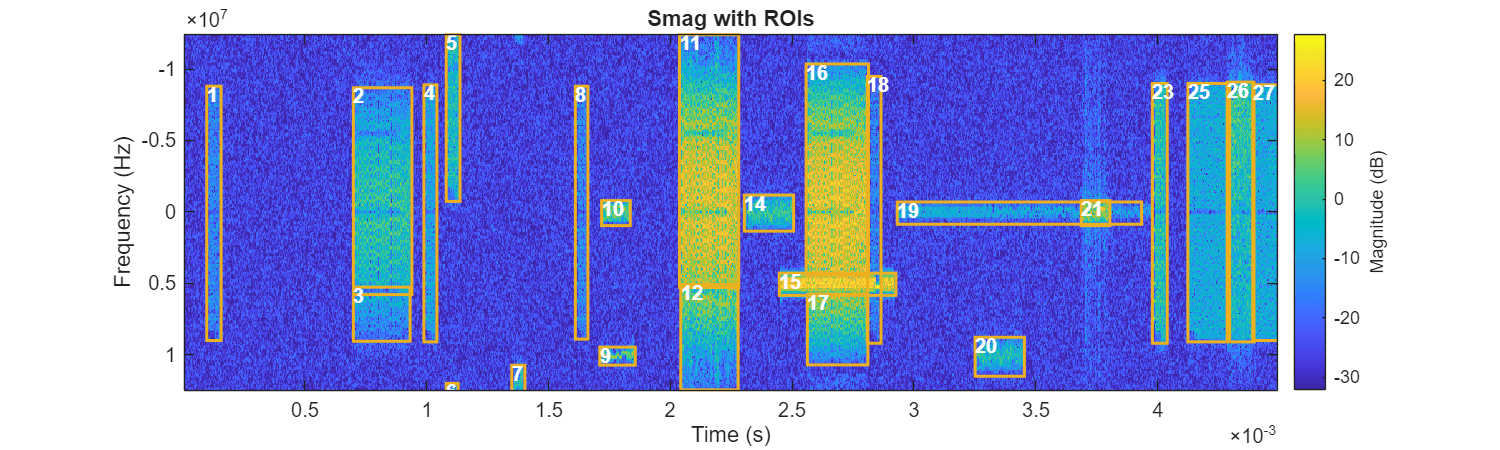
After filtering, the remaining regions are significantly improved when compared to the adaptive gray-scale threshold approach. You may still notice some imperfections, such as regions 16 and 17, which should belong to the same signal but are split into two parts by region 15 in the middle. The results are nearly as accurate as manual labeling and do not require additional expert knowledge.
Evaluating Detection Performance
Besides visually intuitive assessments of accuracy, quantitative evaluation metrics are desirable. Fortunately, the dataset contains signals generated and transmitted under controlled conditions, providing access to the ground truth. Then, by treating ROI localization as a binary classification problem—determining whether a point contains the expected signal—it is possible to easily evaluate the localization results using a confusion matrix.
Load Ground Truth Labels
The complete dataset includes the following six different types of signals. Not all six types are necessarily present in each observation:
BLE 1 MHz: Bluetooth Low Energy signal with 1 MHz bandwidth for low-power, short-range communication
BLE 2 MHz: Bluetooth Low Energy signal with 2 MHz bandwidth for faster data transmission
BT Classic: Traditional Bluetooth for wireless audio, data transfer, and peripheral connectivity
WLANWBG: Wi-Fi operating in wideband mode, typically 802.11ac (Wi-Fi 5) for high data rates
WLANWN: Wi-Fi using 802.11n standard, supporting MIMO for improved range and throughput
WLANWAC: Wi-Fi 802.11ac (Wi-Fi 5) for high-speed data transfer using wider channels and multiple spatial streams
Plot the actual labels of this observation. In this case there are a total of five types of signals.
ROITableTruth = helperReadTrueLabels(filepath);
figure(Position=[0 0 1000 300])
helperPlotROIs(Smag,f,t,ROITableTruth,Class=ROITableTruth{:,"Class"})
title("Ground-Truth Labels")
Calculate Pixel Accuracy of Detected Regions
Convert the localization results into a binary mask and compare it with the ground truth.
[H,W] = size(Smag);
predictedMaskThresh = helperBoundingBoxesToMask(ROITableThreshSelect.BoundingBox,W,H);
predictedMaskSAM = helperBoundingBoxesToMask(ROITableSAMSelect.BoundingBox,W,H);
trueMask = helperBoundingBoxesToMask(ROITableTruth.BoundingBox,W,H);
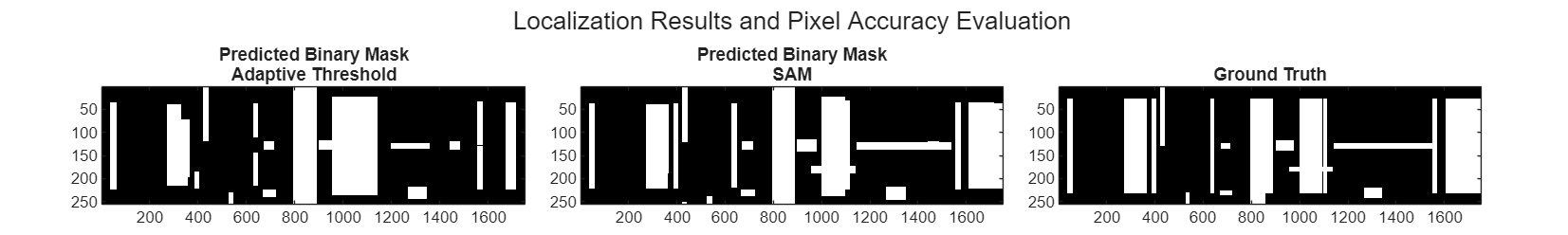
Visualize the results. Here white regions indicate detected signal areas and black regions represent the background.
figure(Position=[0 0 2000 300])
tiled_layout = tiledlayout(1,3,TileSpacing="compact",Padding="compact");
title(tiled_layout,"Localization Results and Pixel Accuracy Evaluation");
nexttile
imagesc(predictedMaskThresh)
title(["Predicted Binary Mask" "Adaptive Threshold"])
nexttile
imagesc(predictedMaskSAM)
title(["Predicted Binary Mask" "SAM"])
nexttile
imagesc(trueMask)
title("Ground Truth")
colormap("gray")
Use a confusion matrix to quantitatively assess accuracy.
figure(Position=[0 0 1000 300])
tiledlayout(1,2)
nexttile
helperPlotConfusionMatrix(predictedMaskThresh,trueMask);
title(["Pixel Accuracy" "Adaptive Threshold"])
nexttile
helperPlotConfusionMatrix(predictedMaskSAM,trueMask);
title(["Pixel Accuracy" "SAM"])
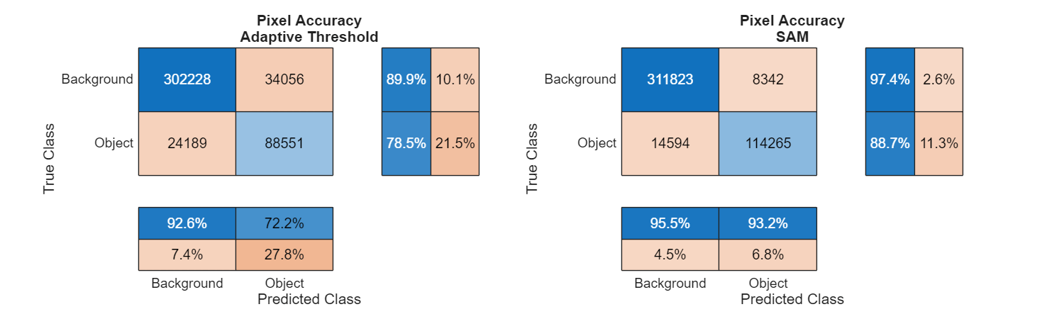
The SAM network method clearly demonstrates higher accuracy, with all metrics approaching 90% or higher level.
Manual Correction of ROIs
The results of unsupervised segmentation and localization cannot be guaranteed to be perfect. The quality of the results depends on various factors, such as the signal itself (for example, signal-to-noise ratio) and the specific objectives, including the definition of the signal and background. Therefore, manual inspection and correction are necessary.
In a real scenario, an expert would manually correct the regions, for example, using the Signal Labeler app. However here for convenience, this example assumes that all the regions are corrected by using the ground truth regions. This assumption serves as the starting point for the next clustering step.
ROITableCorrected = helperCorrectROIs(filepath);
ROI Clustering
Once all regions of interest are corrected, the next step is to label the type of signal contained in each region. This is another nontrivial task that can be as time-consuming as the ROI identification step, especially when processing a large dataset. A way to automate labeling regions of interest as belonging to a particular signal type is to perform clustering. Clustering is a method that groups similar data points based on shared features, enabling regions with similar characteristics to be identified and labeled efficiently. By using clustering, you can significantly reduce the manual effort needed for signal classification, especially when dealing with complicated or high-volume data.
To perform clustering, you need to find relevant features for each region that help define the type of signal they contain. Some intuitive statistics, such as the region's length and width—which correspond to time duration and bandwidth in the signal context—can be useful. Additionally, you can also utilize higher-order time-frequency spectral descriptors like spectral spread, spectral skewness, and spectral entropy. For more information about spectral descriptors, see Spectral Descriptors (Audio Toolbox).
Use the helper function helperExtractFeatures to extract the features mentioned above. This function takes the ROI table and the spectrogram magnitude as inputs and returns an updated table with additional columns for the extracted features
ROITableCorrected = helperExtractFeatures(ROITableCorrected, ...
    TFMap=Smag, ...
    FreqVec=f, ...
    Duration=1, ...
    Bandwidth=1, ...
    CentralFrequency=1, ...
    Spread=1, ...
    Skewness=1, ...
    Kurtosis=1, ...
    Entropy=1);
disp(ROITableCorrected)
    Index     Area                 BoundingBox                     Class                              BoundingBoxTF                          Duration     CentralFrequency    Bandwidth       Spectrum       Centroid        Spread       Skewness      Entropy    Kurtosis
    _____    ______    ____________________________________    ______________    _______________________________________________________    __________    ________________    __________    ____________    ___________    __________    ___________    _______    ________

      1      4237.9    38.433      25.7    20.612     205.6    {'WLANWN'    }     9.984e-05    -9.9609e+06     5.2737e-05          2e+07    5.2737e-05            39062            2e+07    1×256 double         5576.7    5.2778e+06    -0.00073364     11.556      22415
      2       18622    273.37      25.7    90.572     205.6    {'WLANWBG'   }    0.00070144    -9.9609e+06     0.00023173          2e+07    0.00023173            39062            2e+07    1×256 double          18925    4.0105e+06      0.0060434     9.8446      22587
      3      3606.4    386.02      25.7    17.541     205.6    {'WLANWN'    }    0.00099072    -9.9609e+06     4.4878e-05          2e+07    4.4878e-05            39062            2e+07    1×256 double          29015    5.1451e+06      -0.014203     11.786      17548
      4      2429.3    421.77         1    19.053     127.5    {'WLANWN'    }     0.0010829    -1.2402e+07     4.8748e-05     1.2403e+07    4.8748e-05       -6.201e+06       1.2403e+07    1×256 double     -6.666e+06    3.1993e+06      -0.035285     8.3286     6082.3
      5      393.53    527.12     231.3    15.935    24.696    {'WLANWN'    }     0.0013517     1.0059e+07      4.077e-05     2.4023e+06     4.077e-05        1.126e+07       2.4023e+06    1×256 double     1.1742e+07     5.788e+05       -0.86523     2.0322     406.41
      6      3276.2    628.91      25.7    15.935     205.6    {'WLANWN'    }     0.0016128    -9.9609e+06      4.077e-05          2e+07     4.077e-05            39062            2e+07    1×256 double          41053    5.2453e+06      -0.014002     12.235      17125
      7         540    668.48    226.16    52.528     10.28    {'BT_classic'}     0.0017126     9.5703e+06      0.0001344          1e+06     0.0001344        1.007e+07            1e+06    1×256 double     1.0023e+07    2.0546e+05       0.091171     1.0225     83.554
      8      423.31    672.09    123.36    41.178     10.28    {'BT_classic'}     0.0017229    -4.8828e+05     0.00010535          1e+06    0.00010535            11718            1e+06    1×256 double         9210.9    3.2031e+05        0.14847    0.80899     169.37
      9      1547.6    795.97     231.3    62.663    24.696    {'WLANWN'    }     0.0020403     1.0059e+07     0.00016033     2.4023e+06    0.00016033        1.126e+07       2.4023e+06    1×256 double     1.1065e+07    7.2199e+05        0.33668     2.2099     475.57
     10       18622    796.17      25.7    90.572     205.6    {'WLANWBG'   }     0.0020403    -9.9609e+06     0.00023173          2e+07    0.00023173            39062            2e+07    1×256 double     -2.365e+05     4.139e+06       0.050177     9.9081      24371
     11      1521.7    901.04    118.22    74.014     20.56    {'BLE_2MHz'  }     0.0023091    -9.7656e+05     0.00018937          2e+06    0.00018937            23438            2e+06    1×256 double          44145    4.9968e+05      -0.028472     1.8458     380.43
     12      1866.7    955.78    174.76    181.58     10.28    {'BLE_1MHz'  }     0.0024499     4.5898e+06     0.00046458          1e+06    0.00046458       5.0898e+06            1e+06    1×256 double     5.0274e+06    2.5747e+05        0.08976     0.8666      122.2
     14       19443    998.97      25.7    94.563     205.6    {'WLANWBG'   }       0.00256    -9.9609e+06     0.00024194          2e+07    0.00024194            39062            2e+07    1×256 double     3.5632e+05    4.0359e+06       -0.11932     10.853      12228
     15      3282.6    1097.8      25.7    15.966     205.6    {'WLANWN'    }     0.0028134    -9.9609e+06     4.0849e-05          2e+07    4.0849e-05            39062            2e+07    1×256 double     3.6853e+06    3.5223e+06        -2.1162     2.3482     393.63
     17      4174.6    1142.9    123.36    406.08     10.28    {'BLE_1MHz'  }     0.0029286    -4.8828e+05       0.001039          1e+06      0.001039            11718            1e+06    1×256 double         2164.6    2.9671e+05        0.16747    0.88593     165.05
     18      1521.7    1269.4    221.02    74.014     20.56    {'BLE_2MHz'  }     0.0032512      9.082e+06     0.00018937          2e+06    0.00018937       1.0082e+07            2e+06    1×256 double     1.0081e+07    4.9872e+05       0.021384     1.8438     381.88
     20      423.31    1439.2    123.36    41.178     10.28    {'BT_classic'}     0.0036864    -4.8828e+05     0.00010535          1e+06    0.00010535            11718            1e+06    1×256 double        -7040.2    3.1547e+05        0.22032    0.91686     159.53
     21      3917.4    1552.2      25.7    19.053     205.6    {'WLANWN'    }     0.0039757    -9.9609e+06     4.8748e-05          2e+07    4.8748e-05            39062            2e+07    1×256 double          15269      5.08e+06      -0.005948      11.86      14657
     22       30342    1606.4      25.7    147.58     205.6    {'WLANWN'    }     0.0041139    -9.9609e+06     0.00037758          2e+07    0.00037758            39062            2e+07    1×256 double    -5.1597e+05    5.3281e+06        0.14039     10.577      25602
     24      8081.6    1671.6      25.7    39.307     205.6    {'WLANWN'    }     0.0042829    -9.9609e+06     0.00010057          2e+07    0.00010057            39062            2e+07    1×256 double    -1.1865e+06    5.2865e+06        0.32441     11.982      17707
Once all features are calculated and stored in the table, you can try different combinations of features to determine the best set. This selection often depends on prior knowledge, observation, and experimentation. The final subset of features chosen here is as follows.
featureList = {'Duration','Spread','Skewness','Entropy'};Extract the selected features from the table as a feature matrix for the next clustering step. Because different features usually have very inconsistent numerical dynamic ranges, normalize each feature to maintain relative balance.
featureMatrix = ROITableCorrected{:,featureList};
featureMatrixNorm = normalize(featureMatrix,1,"zscore");
Determining the number of clusters for clustering algorithms is a complicated issue.
Although we know there are at most six types of signals, the specific number present in a given observation is unknown.
From the ground truth, we can see that some signals are incomplete due to limitations in sampling frequency and duration, such as regions 5 and 4.
Overlaps exist between some regions, potentially affecting any features due to interference from overlapping areas, such as regions 17 and 20 as well as regions 15 and 12.
These factors lead to inconsistencies in the features of even the same type of signals within the same observation. Such challenges increase the difficulty in determining the correct number of clusters. To address these challenges, you can employ proactive overclustering, setting the number of clusters higher than the actual number of clusters needed. This intentional redundancy in clusters helps to accommodate anomalous points in separate cluster grouped and avoid normal points being clustered incorrectly.
In this case, over-clustering allows you to cluster in a more meaningful way by identifying substructures. Choose 7 as the cluster number.
nClasses = 7;
The k-medoids clustering algorithm groups data points by minimizing the distance between each point and a selected representative point, called a medoid, which is an actual point in the dataset. Unlike k-means, which uses the average as the cluster center, k-medoids is more robust to outliers, making it suitable for datasets where the mean is not meaningful. Here, we apply k-medoids with a "cityblock" distance to divide our data into clusters, iterating until clusters stabilize.
rng("default")
[classes,C] = kmedoids(featureMatrixNorm,nClasses, ...
    Replicates=1000,Distance="cityblock");
ROITableCorrected.Class = classes;
figure(Position=[0 0 1000 300])
helperPlotROIs(Smag,f,t,ROITableCorrected,Classes=classes);
Different areas have been divided into 7 categories. Meaningful distribution patterns between different clusters and signals are already evident, although the labels for each category are currently numeric placeholders without actual meaning. After identifying 7 clusters, manually assign labels to each cluster that correspond to meaningful real-world signal categories. This step, especially when dealing with long observation periods containing numerous regions, is much easier than classifying each region individually because it allows for batch labeling by cluster.
For example, an expert might observe that regions 10 and 14 are clearly WLANWBG signals, so they assign cluster label 1 to WLANWBG. Then, upon seeing region 24, the expert identifies it as another distinct signal type and assigns the appropriate label. This process continues, with any extra or ambiguous clusters carefully assigned to one of the existing labels based on their characteristics. After this initial assignment, only minimal in-cluster adjustments are typically needed to ensure accurate labeling.
Quantitatively Evaluate the Clustering Results
Next, you quantitatively assess the clustering results by using ground truth data to simulate the expert decision-making process. This process mimics the logic of manual labeling based on clustering results. For each cluster, the helperMapClusterLabels function assigns the closest signal name by examining all signals within the cluster and identifying the type that is most represented, thus determining the true signal type name for each cluster. Using ground truth in this way helps bridge clustering results with expert-like manual labeling, ensuring each cluster accurately reflects a meaningful signal type
trueLabels = ROITableTruth.Class;
predictedLabels = arrayfun(@(x) num2str(x),classes,UniformOutput=false);
predictedLabelsMapped = helperMapClusterLabels(trueLabels,predictedLabels);
Replace the cluster index with the final determined signal type label. Then, compare it with the ground truth.
figure(Position=[0 0 1000 300])
helperPlotROIs(Smag,f,t,ROITableCorrected,Classes=predictedLabelsMapped);
title("Clustering Results")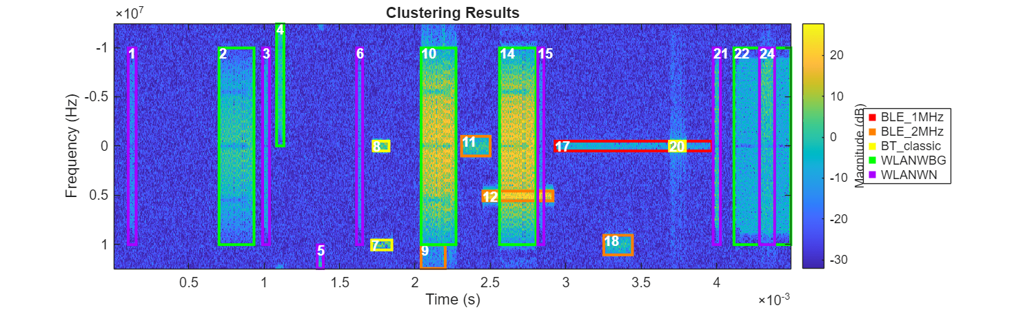
figure(Position=[0 0 1000 300])
helperPlotROIs(Smag,f,t,ROITableCorrected,Classes=trueLabels);
title("Ground Truth")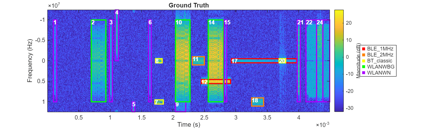
After assigning signal category labels to each cluster, only several regions are mistakenly classified into the wrong groups. It is understandable that clustering algorithms have difficulties in identifying overlapping areas like region 12 or incomplete regions such as regions 4 and 9. This is mainly because the time-frequency characteristics of these regions are significantly disrupted due to their incompleteness or overlap.
figure
confChart = confusionchart(trueLabels,predictedLabelsMapped);
confChart.Title = "Confusion Matrix of Class Predictions";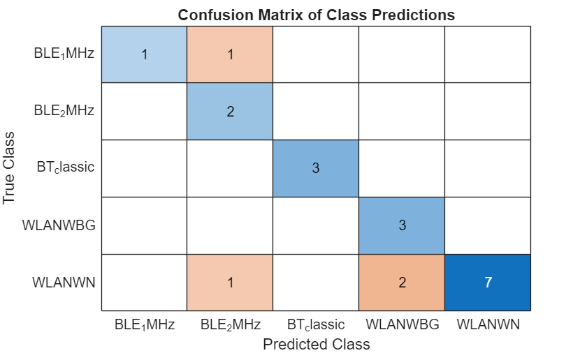
It is possible to further increase the number of clusters to separate more outlier regions affected by truncation and overlap into independent groups, potentially improving accuracy. However, increasing the number of clusters would also raise the workload for determining the signal categories of each cluster, creating a tradeoff.
Explore More Cases
Using the same method, without any parameter changes, repeat the above clustering steps to perform assisted classification on more cases. Then, observe the results. Retrieve all signals from the dataset, excluding the one used for the demonstration above.
fileList = string({dir(fullfile(pwd,"TFLabeling","*.mat")).name});
fileList(fileList == filename) = [];
fig = figure; fig.Position=[0 0 8000 4000]; tl = tiledlayout(5,5,TileSpacing="tight",Padding="tight"); for i = 1:length(fileList) filename = fileList{i}; filepath = fullfile(datafolder,filename); file = load(filepath); sig = file.complex_array'; fs = 25e6; win = hann(256); [S,f,t] = stft(sig,fs,FrequencyRange="centered",Window=win); Smagtmp = abs(S); ROITableCorrectedTmp = helperCorrectROIs(filepath); ROITableCorrectedTmp = helperExtractFeatures(ROITableCorrectedTmp, ... TFMap=Smagtmp, ... FreqVec=f, ... Duration=1, ... Spread=1, ... Skewness=1, ... Entropy=1); ROITableTruthTmp = helperReadTrueLabels(filepath); ROITableTruthTmp.SigID = repmat(extractBefore(filename,".mat"),height(ROITableTruthTmp),1); featureList = {'Duration','Spread','Skewness','Entropy'}; featureMatrix = ROITableCorrectedTmp{:,featureList}; featureMatrixNorm = normalize(featureMatrix,1,"zscore"); rng("default") classes = kmedoids(featureMatrixNorm,7, ... Replicates=100,Distance="cityblock"); trueLabels = ROITableTruthTmp.Class; predictedLabels = arrayfun(@(x)num2str(x),classes,UniformOutput=false); predictedLabelsMapped = helperMapClusterLabels(trueLabels,predictedLabels); C = confusionmat(trueLabels,predictedLabelsMapped); nexttile confChart = confusionchart(C,categories(categorical(trueLabels))); nexttile([1 2]) helperPlotROIs(Smagtmp,f,t,ROITableTruthTmp,Classes=trueLabels,Simplify=1); title("Clustering Results") nexttile([1 2]) helperPlotROIs(Smagtmp,f,t,ROITableCorrectedTmp, ... Classes=predictedLabelsMapped,Simplify=1); title("Ground Truth") end
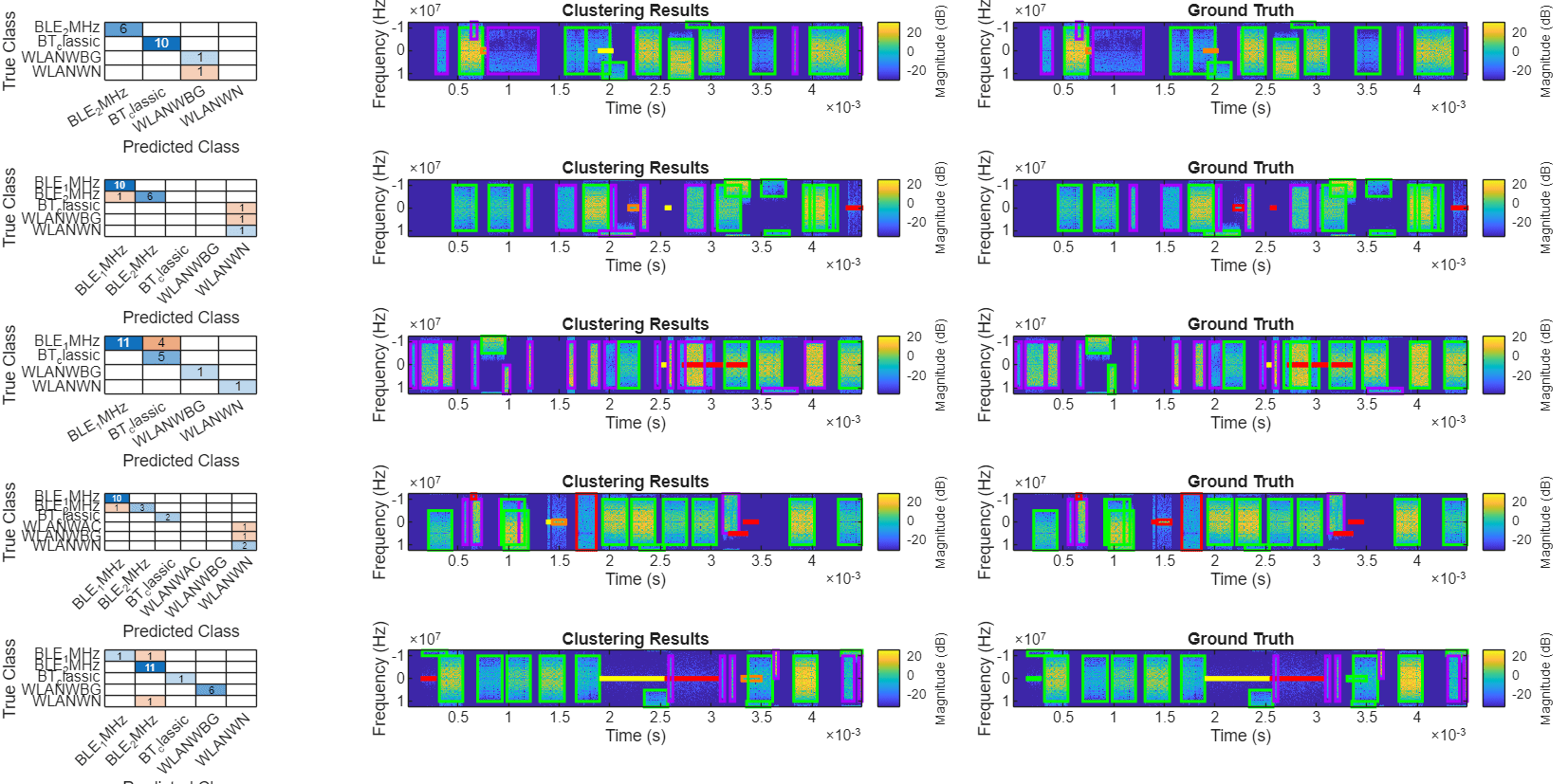
It is evident that the clustering method achieves good results across various cases.
Summary
This example demonstrates how to use AI to automate the labeling of wireless signals in the time-frequency domain. The annotation process requires minimal prior knowledge of the collected signal content, significantly reducing the effort needed for manual annotation. This aspect also makes it exceptionally easy to transfer the process to many other datasets and even different fields.
Reference
[1] Cheng, Cheng, Guijun Ma, Yong Zhang, Mingyang Sun, Fei Teng, Han Ding, and Ye Yuan. “A Deep Learning-Based Remaining Useful Life Prediction Approach for Bearings.” IEEE/ASME Transactions on Mechatronics 25, no. 3 (June 2020): 1243–54.
[2] Kirillov, Alexander, Eric Mintun, Nikhila Ravi, Hanzi Mao, Chloe Rolland, Laura Gustafson, Tete Xiao, Spencer Whitehead, Alexander C. Berg, Wan-Yen Lo, Piotr Dollár and Ross B. Girshick. "Segment Anything." 2023 IEEE/CVF International Conference on Computer Vision (ICCV) (2023): 3992-4003.