Signal Labeler
Label signal attributes, regions, and points of interest
Description
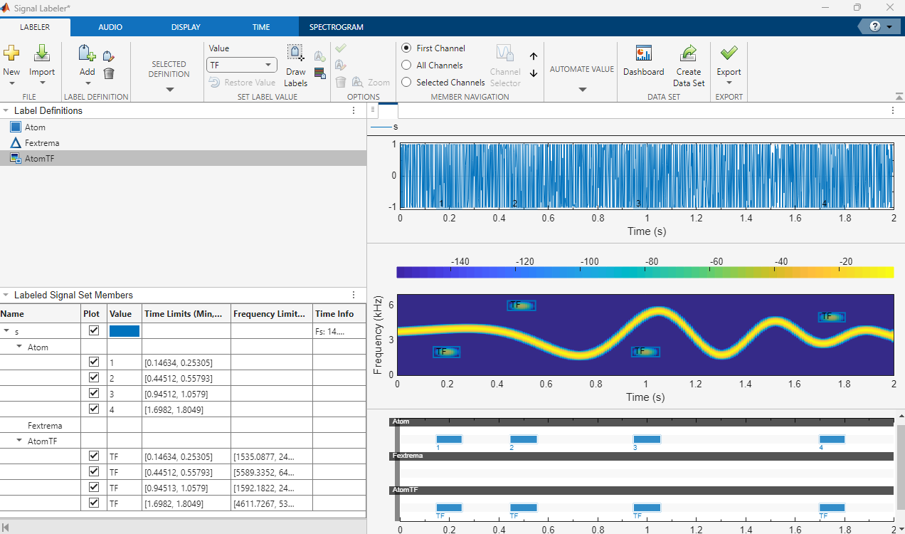
The Signal Labeler app is an interactive tool that enables you to label signals for analysis or for use in machine learning and deep learning applications. Using Signal Labeler, you can:
Label signal attributes, regions, and points of interest
Label spectrogram time-frequency regions of interest (since R2025a)
Use logical, categorical, numerical, or string-valued labels
Automatically label signal peaks or bounded signal regions
Apply custom labeling functions
Import, label, and play audio signals
Use frequency and time-frequency views to aid labeling in time domain
Use time view to aid labeling in time-frequency domain (since R2025a)
Create data sets that include signals, spectrograms, and label masks (since R2025a)
Add, edit, and delete labels or sublabels
Display selected subsets of signals and labels
Signal Labeler saves data as labeledSignalSet
objects. You can export labeledSignalSet objects to MATLAB® or Diagnostic Feature
Designer (Predictive Maintenance Toolbox). You can create data sets as files to train a network, classifier, or analyze
data and report statistics.
For more information, see Use Signal Labeler App.
You need an Audio Toolbox™ license to import, play, and label audio signals.
Audio playback is not supported in MATLAB Online.
You need a Predictive Maintenance Toolbox™ license to export labeled signal sets to Diagnostic Feature Designer.
Signal Labeler no longer supports the feature extraction mode, which is now available as an app. To extract signal features, open Signal Feature Extractor from the MATLAB Toolstrip or the Command Window.
Open the Signal Labeler App
MATLAB Toolstrip: On the Apps tab, under Signal Processing and Audio, click the app icon.
MATLAB command prompt: Enter
signalLabeler.
Examples
This example shows how to track your labeling progress and assess the quality of labels with the Dashboard. In this mode, you can quickly determine how many members are labeled and inspect the distributions of label values and durations in your data set. This step facilitates the process of obtaining complete and accurate data sets for machine learning.
Download and Prepare the Data
Use the QTdownload function to download the electrocardiogram (ECG) signals from the publicly available QT database [1] [2] to a new temporary directory folder. The code for this function is at the end of the example.
folder = QTdownload;
Each file contains an ECG signal ecgSignal, a table of region labels signalRegionLabels, and the sample rate variable Fs. All signals have a sample rate of 250 Hz. The region labels correspond to three heartbeat morphologies:
P wave
QRS complex
T wave
Create a signal datastore that points to folder. Specify the signal variable name ecgSignal and the sample rate variable Fs.
sds = signalDatastore(folder,SignalVariableNames="ecgSignal", ...
    SampleRateVariableName="Fs");
Create a subset of the datastore containing the first twenty files. Use this subset as the source for a labeledSignalSet object.
subsds = subset(sds,1:20);
lss = labeledSignalSet(subsds);
Label Regions of Interest
Open the Signal Labeler app and import the labeled signal set from the workspace. Plot the first signal in the data set. From the Display tab, select the panner and zoom to a smaller region of the signal for better visualization.

From the Labeler tab, define a categorical region-of-interest (ROI) label with P, QRS and T categories. Name the label BeatMorphologies.
Create a custom labeling function labelECGregions to locate and label the three different regions of interest. Code for the custom function appears later in the example. You can save the function in your current folder, on the MATLAB path, or add it in the app by selecting Add Custom Function in the Automate Value gallery. See Custom Labeling Functions for more information.
Select BeatMorphologies in the Label Definitions browser and choose the labelECGregions function from the Automate Value gallery. Select Auto-Label and then Auto-Label and Inspect Plotted. Click Run. From the Display tab, zoom in on a region of the labeled signal and use the panner to navigate through time. If the labeling is satisfactory, click Save Labels to accept the labels and close the Autolabel tab. You can see the labels and their location values in the Labeled Signal Set Members browser.

Visualize Labeling Progress and Statistics
Select the Dashboard in the toolstrip of the Labeler tab. The progress bar shows 5% of members are labeled with at least one ROI label. This corresponds to 1/20 members in the data set. The label distribution pie chart shows the number of instances of each category for the selected label definition.

Close the dashboard and continue your labeling. Select Auto-Label and then Auto-Label All Signals to label the next four signals in the list. Check the box next to the signal names you want to label and then click OK.
Select the Dashboard again. The progress bar now shows 25% of members are labeled. Verify the distribution of each category (P, QRS, or T) is as expected. The Label Distribution pie chart shows that each category makes up about a third of all label instances. Select the Time Distribution histogram chart from the Plots gallery to view the average duration of the P and T waves and QRS complexes, including outliers. Notice the T waves have longer durations than the P waves and QRS complexes.
Display the Member Count chart to better visualize the distribution of labels across members and number of instances. Most members in the data set have between 0–500 instances of P, QRS, and T regions.

Click on the progress bar plot and adjust the Threshold in the toolstrip to count only members with at least 5000 labels. Now only three of the five labeled members are included in the count. Adjust the count threshold to better differentiate between labeled and unlabeled members based on your labeling requirements.

labelECGregions Function
The labelECGregions function uses a pretrained deep learning network to identify P, QRS and T heartbeat morphologies in ECG signals.
function [labelVals,labelLocs] = labelECGregions(x,t,parentLabelVal,parentLabelLoc,varargin)

labelVals = cell(2,1);
labelLocs = cell(2,1);

if nargin < 5
    Fs = 250;
else
    Fs = varargin{1};
end

% Download the pretrained network

netfil = matlab.internal.examples.downloadSupportFile("SPT", ...
    "data/QTDatabaseECGSegmentationNetworks.zip"); %#ok<*UNRCH>
unzip(netfil,fullfile(tempdir,"ECGnet"))
load(fullfile(tempdir,"ECGnet","trainedNetworks.mat"))

    for kj = 1:size(x,2)

        sig = x(:,kj)';

        predTest = classify(rawNet,sig,MiniBatchSize=50);

        msk = signalMask(predTest);
        msk.SpecifySelectedCategories = true;
        msk.SelectedCategories = find(msk.Categories ~= "n/a");

        labels = roimask(msk);
        labelVals{kj} = labels.Value;
        labelLocs{kj} = labels.ROILimits/Fs;

    end

labelVals = vertcat(labelVals{:});
labelLocs = cell2mat(labelLocs);

end
QTdownload Function
You can download the data files from https://www.mathworks.com/supportfiles/SPT/data/QTDatabaseECGData.zip or use the unzip function to create a folder in your temporary directory with 210 MAT files in it.
function folder = QTdownload

localfile = matlab.internal.examples.downloadSupportFile("SPT", ...
    "data/QTDatabaseECGData1.zip");
unzip(localfile,tempdir)
folder = fullfile(tempdir,"QTDataset");

end
References
[1] Goldberger, Ary L., Luis A. N. Amaral, Leon Glass, Jeffery M. Hausdorff, Plamen Ch. Ivanov, Roger G. Mark, Joseph E. Mietus, George B. Moody, Chung-Kang Peng, and H. Eugene Stanley. "PhysioBank, PhysioToolkit, and PhysioNet: Components of a New Research Resource for Complex Physiologic Signals." Circulation. Vol. 101, No. 23, 2000, pp. e215–e220. [Circulation Electronic Pages; http://circ.ahajournals.org/content/101/23/e215.full].
[2] Laguna, Pablo, Roger G. Mark, Ary L. Goldberger, and George B. Moody. "A Database for Evaluation of Algorithms for Measurement of QT and Other Waveform Intervals in the ECG." Computers in Cardiology. Vol.24, 1997, pp. 673–676.
Related Examples
- Label Signal Attributes, Regions of Interest, and Points
- Examine Labeled Signal Set
- Automate Signal Labeling with Custom Functions
- Label Spoken Words in Audio Signals
- Label Radar Signals with Signal Labeler (Radar Toolbox)
- Export Labeled Data from Signal Labeler for AI-Based Spectrum Sensing Applications
Programmatic Use
Version History
Introduced in R2019aSee Also
Apps
Functions
Topics
- Use Signal Labeler App
- Import Data into Signal Labeler
- Import and Play Audio File Data in Signal Labeler
- Create or Import Signal Label Definitions
- Label Signals Interactively or Automatically
- Custom Labeling Functions
- Customize Labeling View
- Spectrogram Computation in Signal Labeler
- Dashboard
- Export Data and Create Data Sets
- Signal Labeler Usage Tips