stftLayer

Short-time Fourier transform layer

Since R2021b

Description

An STFT layer computes the short-time Fourier transform of the input. Use of this layer requires Deep Learning Toolbox™.

Creation

Syntax

layer = stftLayer

layer = stftLayer(PropertyName=Value)

Description

layer = stftLayer creates a Short-Time Fourier Transform (STFT) layer. The input to stftLayer must be a real-valued dlarray (Deep Learning Toolbox) object in "CBT" format with a size along the time dimension greater than the length of Window. stftLayer formats the output as "SCBT". For more information, see Layer Output Format.

Note

When you initialize the learnable parameters of stftLayer, the layer weights are set to the analysis window used to compute the transform. It is not recommended to initialize the weights directly.

layer = stftLayer(PropertyName=Value) sets properties using one or more name-value arguments. You can specify the analysis window and the number of overlapped samples, among others.

Note

You cannot use this syntax to set the Weights property.

Properties

STFT

Window — Analysis window

Read-only: hann(128,'periodic') (default) | vector

This property is read-only.

Analysis window used to compute the STFT, specified as a vector with two or more elements.

Example: (1-cos(2*pi*(0:127)'/127))/2 and hann(128) both specify a Hann window of length 128.

Data Types: double | single

OverlapLength — Number of overlapped samples

Read-only: 96 (default) | positive integer

This property is read-only.

Number of overlapped samples, specified as a positive integer strictly smaller than the length of Window.

The stride between consecutive windows is the difference between the window length and the number of overlapped samples.

Data Types: double | single

FFTLength — Number of DFT points

Read-only: 128 (default) | positive integer

This property is read-only.

Number of frequency points used to compute the discrete Fourier transform, specified as a positive integer greater than or equal to the window length. If not specified, this argument defaults to the length of the window.

Data Types: double | single

TransformMode — Layer transform mode

"mag" (default) | "squaremag" | "logmag" | "logsquaremag" | "realimag"

Layer transform mode, specified as one of these:

• "mag" — STFT magnitude

• "squaremag" — STFT squared magnitude

• "logmag" — Natural logarithm of the STFT magnitude

• "logsquaremag" — Natural logarithm of the STFT squared magnitude

• "realimag" — Real and imaginary parts of the STFT, concatenated along the channel dimension

Data Types: char | string

Layer

Weights — Layer weights

[] (default) | numeric array | dlarray object

Layer weights, specified as [], a numeric array, or a dlarray object.

The layer weights are learnable parameters. You can use initialize (Deep Learning Toolbox) to initialize the learnable parameters of a dlnetwork (Deep Learning Toolbox) that includes stftLayer objects. When you initialize the layers, initialize sets Weights to the analysis window used to compute the transform. For more information, see Initialize Short-Time Fourier Transform Layer. (since R2025a)

It is not recommended to initialize the weights directly.

Data Types: double | single

WeightLearnRateFactor — Multiplier for weight learning rate

0 (default) | nonnegative scalar

Multiplier for weight learning rate, specified as a nonnegative scalar. If not specified, this property defaults to zero, resulting in weights that do not update with training. You can also set this property using the setLearnRateFactor (Deep Learning Toolbox) function.

Data Types: double | single

Name — Layer name

'' (default) | character vector | string scalar

Layer name, specified as a character vector or a string scalar. For Layer array input, the trainnet (Deep Learning Toolbox) and dlnetwork (Deep Learning Toolbox) functions automatically assign names to unnamed layers.

The stftLayer object stores this property as a character vector.

Data Types: char | string

NumInputs — Number of inputs

Read-only: 1 (default)

This property is read-only.

Number of inputs to the layer, stored as 1. This layer accepts a single input only.

Data Types: double

InputNames — Input names

Read-only: {'in'} (default)

This property is read-only.

Input names, stored as {'in'}. This layer accepts a single input only.

Data Types: cell

NumOutputs — Number of outputs

Read-only: 1 (default)

This property is read-only.

Number of outputs from the layer, stored as 1. This layer has a single output only.

Data Types: double

OutputNames — Output names

Read-only: {'out'} (default)

This property is read-only.

Output names, stored as {'out'}. This layer has a single output only.

Data Types: cell

Examples

Short-Time Fourier Transform of Chirp

Generate a signal sampled at 600 Hz for 2 seconds. The signal consists of a chirp with sinusoidally varying frequency content. Store the signal in a deep learning array with "CTB" format.

fs = 6e2; 
x = vco(sin(2*pi*(0:1/fs:2)),[0.1 0.4]*fs,fs);

dlx = dlarray(x,"CTB");

Create a short-time Fourier transform layer with default properties. Create a dlnetwork object consisting of a sequence input layer and the short-time Fourier transform layer. Specify a minimum sequence length of 128 samples. Run the signal through the predict method of the network.

ftl = stftLayer;

dlnet = dlnetwork([sequenceInputLayer(1,MinLength=128) ftl]);
netout = predict(dlnet,dlx);

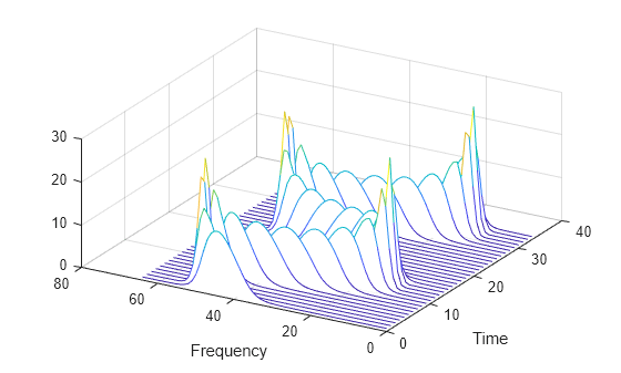
Convert the network output to a numeric array. Use the squeeze function to remove the length-1 channel and batch dimensions. Plot the magnitude of the STFT. The first dimension of the array corresponds to frequency and the second to time.

q = extractdata(netout);

waterfall(squeeze(q)')
set(gca,XDir="reverse",View=[30 45])
xlabel("Frequency")
ylabel("Time")

Short-Time Fourier Transform of Sinusoid

Generate a 3 × 160 (× 1) array containing one batch of a three-channel, 160-sample sinusoidal signal. The normalized sinusoid frequencies are π/4 rad/sample, π/2 rad/sample, and 3π/4 rad/sample. Save the signal as a dlarray, specifying the dimensions in order. dlarray permutes the array dimensions to the "CBT" shape expected by a deep learning network.

nch = 3;
N = 160;
x = dlarray(cos(pi.*(1:nch)'/4*(0:N-1)),"CTB");

Create a short-time Fourier transform layer that can be used with the sinusoid. Specify a 64-sample rectangular window, 48 samples of overlap between adjoining windows, and 1024 DFT points. By default, the layer outputs the magnitude of the STFT.

stfl = stftLayer(Window=rectwin(64), ...
    OverlapLength=48, ...
    FFTLength=1024);

Create a two-layer dlnetwork object containing a sequence input layer and the STFT layer you just created. Treat each channel of the sinusoid as a feature. Specify the signal length as the minimum sequence length for the input layer.

layers = [sequenceInputLayer(nch,MinLength=N) stfl];
dlnet = dlnetwork(layers);

Run the sinusoid through the forward method of the network.

dataout = forward(dlnet,x);

Convert the network output to a numeric array. Use the squeeze function to collapse the size-1 batch dimension. Permute the channel and time dimensions so that each array page contains a two-dimensional spectrogram. Plot the STFT magnitude separately for each channel in a waterfall plot.

q = squeeze(extractdata(dataout));
q = permute(q,[1 3 2]);

for kj = 1:nch
    subplot(nch,1,kj)
    waterfall(q(:,:,kj)')
    view(30,45)
    zlabel("Ch. "+string(kj))
end

Initialize Short-Time Fourier Transform Layer

Since R2025a

Initialize short-time Fourier transform (STFT) layer weights to window, update deep learning neural network, and reset learnable parameters.

Define an array of seven layers: a sequence input layer, an STFT layer, a 2-D convolutional layer, a batch normalization layer, a rectified linear unit (ReLU) layer, a fully connected layer, and a softmax layer. There is one feature in the sequence input. Set the minimum signal length in the sequence input layer to 512 samples. For the STFT layer, use a 256-sample Hamming window and an overlap length of 128 samples.

win = hamming(256);
layers = [
   sequenceInputLayer(1,MinLength=512)
   stftLayer(Window=win,OverlapLength=128,Name="stft")
   convolution2dLayer(4,16,Padding="same")
   batchNormalizationLayer
   reluLayer
   fullyConnectedLayer(3)
   softmaxLayer];

Create a deep learning neural network from the layer array. By default, the dlnetwork function initializes the network at creation. For reproducibility, use the default random number generator.

rng("default")
net = dlnetwork(layers);

Display the table of learnable parameters. The network weights and bias are nonempty dlarray objects.

tInit1 = net.Learnables

tInit1=7×3 table
       Layer       Parameter           Value        
    ___________    _________    ____________________

    "stft"         "Weights"    {256×1      dlarray}
    "conv"         "Weights"    {  4×4×1×16 dlarray}
    "conv"         "Bias"       {  1×1×16   dlarray}
    "batchnorm"    "Offset"     {  1×16     dlarray}
    "batchnorm"    "Scale"      {  1×16     dlarray}
    "fc"           "Weights"    {  3×2064   dlarray}
    "fc"           "Bias"       {  3×1      dlarray}

Compare the initialized weights of the STFT layer from the list of learnable parameters with the Window property of the STFT layer. The stftLayer weights are single precision and initialized to the specified window.

isequal(tInit1.Value{1},single(net.Layers(2).Window))

ans = logical
   1

Set the learnable parameters to empty arrays.

net = dlupdate(@(x)[],net);
net.Learnables

ans=7×3 table
       Layer       Parameter       Value    
    ___________    _________    ____________

    "stft"         "Weights"    {0×0 double}
    "conv"         "Weights"    {0×0 double}
    "conv"         "Bias"       {0×0 double}
    "batchnorm"    "Offset"     {0×0 double}
    "batchnorm"    "Scale"      {0×0 double}
    "fc"           "Weights"    {0×0 double}
    "fc"           "Bias"       {0×0 double}

Reinitialize the network. Display the network and the learnable parameters. The network weights and bias are nonempty dlarray objects.

net = initialize(net);
tInit2 = net.Learnables

tInit2=7×3 table
       Layer       Parameter           Value        
    ___________    _________    ____________________

    "stft"         "Weights"    {256×1      dlarray}
    "conv"         "Weights"    {  4×4×1×16 dlarray}
    "conv"         "Bias"       {  1×1×16   dlarray}
    "batchnorm"    "Offset"     {  1×16     dlarray}
    "batchnorm"    "Scale"      {  1×16     dlarray}
    "fc"           "Weights"    {  3×2064   dlarray}
    "fc"           "Bias"       {  3×1      dlarray}

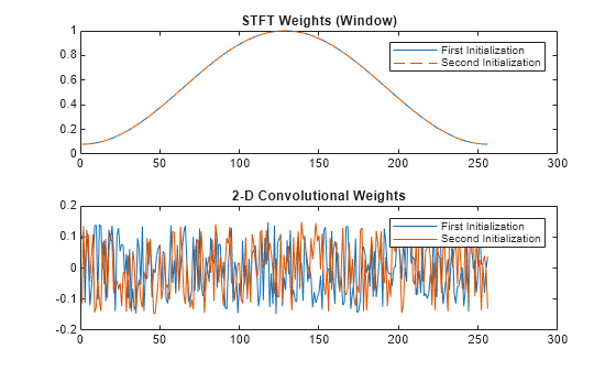
Compare the weights from the STFT and 2-D convolutional layers along the two initialization calls. The STFT layer sets the weights using the specified window, while the convolutional layer weights consists of a new set of random values.

tiledlayout flow
nexttile
plot(tInit1.Value{1})
hold on
plot(tInit2.Value{1},"--")
hold off
title("STFT Weights (Window)")
legend(["First" "Second"] + " Initialization")
nexttile
plot([tInit1.Value{2}(:) tInit2.Value{2}(:)])
title("2-D Convolutional Weights")
legend(["First" "Second"] + " Initialization")

More About

Short-Time Fourier Transform

The short-time Fourier transform (STFT) is used to analyze how the frequency content of a nonstationary signal changes over time. The magnitude squared of the STFT is known as the spectrogram time-frequency representation of the signal. For more information about the spectrogram and how to compute it using Signal Processing Toolbox™ functions, see Spectrogram Computation with Signal Processing Toolbox.

The STFT of a signal is computed by sliding an analysis window g(n) of length M over the signal and calculating the discrete Fourier transform (DFT) of each segment of windowed data. The window hops over the original signal at intervals of R samples, equivalent to L = M – R samples of overlap between adjoining segments. Most window functions taper off at the edges to avoid spectral ringing. The DFT of each windowed segment is added to a complex-valued matrix that contains the magnitude and phase for each point in time and frequency. The STFT matrix has

$$k=\lfloor \frac{N_x-L}{M-L}\rfloor$$

columns, where N_x is the length of the signal x(n) and the ⌊⌋ symbols denote the floor function. The number of rows in the matrix equals N_DFT, the number of DFT points, for centered and two-sided transforms and an odd number close to N_DFT/2 for one-sided transforms of real-valued signals.

The mth column of the STFT matrix $$X(f)=\left[\begin{array}{ccccc}{X}_1(f)& X_2(f)& X_3(f)& \cdots & X_k(f)\end{array}\right]$$ contains the DFT of the windowed data centered about time mR:

$$X_m(f)={\displaystyle \sum _{n=-\infty }^{\infty }x(n)g(n-mR)e^{-j2\pi fn}}.$$

Layer Output Format

stftLayer formats the output as "SCBT", a sequence of 1-D images where the image height corresponds to frequency, the second dimension corresponds to channel, the third dimension corresponds to batch, and the fourth dimension corresponds to time.

• You can feed the output of stftLayer unchanged to a 1-D convolutional layer when you want to convolve along the frequency ("S") dimension. For more information, see convolution1dLayer (Deep Learning Toolbox).

• To feed the output of stftLayer to a 1-D convolutional layer when you want to convolve along the time ("T") dimension, you must place a flatten layer after the stftLayer. For more information, see flattenLayer (Deep Learning Toolbox).

• You can feed the output of stftLayer unchanged to a 2-D convolutional layer when you want to convolve along the frequency ("S") and time ("T") dimensions. For more information, see convolution2dLayer (Deep Learning Toolbox).

• To use stftLayer as part of a recurrent neural network, you must place a flatten layer after the stftLayer. For more information, see lstmLayer (Deep Learning Toolbox) and gruLayer (Deep Learning Toolbox).

• To use the output of stftLayer with a fully connected layer as part of a classification workflow, you must reduce the time ("T") dimension of the output so that it has size 1. To reduce the time dimension of the output, place a global pooling layer before the fully connected layer. For more information, see globalAveragePooling2dLayer (Deep Learning Toolbox) and fullyConnectedLayer (Deep Learning Toolbox).

Extended Capabilities

C/C++ Code Generation

Generate C and C++ code using MATLAB® Coder™. (since R2025a)

Usage notes and limitations:

• You can generate generic C/C++ code that does not depend on third-party libraries and deploy the generated code to hardware platforms.

GPU Code Generation

Generate CUDA® code for NVIDIA® GPUs using GPU Coder™. (since R2025a)

Usage notes and limitations:

• You can generate CUDA code that is independent of deep learning libraries and deploy the generated code to platforms that use NVIDIA^® GPU processors.

Version History

Introduced in R2021b

R2025a: Initialize layer weights through dlnetwork initialization

Starting in R2025a, you can use initialize (Deep Learning Toolbox) to initialize learnable parameters for deep learning neural networks that include stftLayer objects.

R2025a: New Weights default value

Starting in R2025a, the default value of the Weights property is []. Prior to R2025a, stftLayer set the default value to the analysis window used to compute the transform.

R2025a: C/C++ and GPU Code Generation

The stftLayer object supports:

• C/C++ code generation. You must have MATLAB^® Coder™ to generate C/C++ code.

• Code generation for NVIDIA GPUs. You must have GPU Coder™ to generate GPU code.

R2023b: Weights initialized to analysis window

Starting in R2023b, stftLayer initializes the Weights learnable parameter to the analysis window used to compute the transform. Previously, the parameter was initialized to an array containing the Gabor atoms for the STFT.

R2022b: OutputMode property to be removed in a future release

The OutputMode property of stftLayer will be removed in a future release. Update your code and networks to make them compatible with stftLayer output in "SCBT" format. For more information, see Layer Output Format.