hampel
Outlier removal using Hampel identifier
Syntax
Description
y = hampel(x)x to detect and remove outliers. For each
sample of x, the function computes the median of a window composed of
the sample and its six surrounding samples, three per side. It also estimates the standard
deviation of each sample about its window median using the median absolute deviation. If a
sample differs from the median by more than three standard deviations, it is replaced with
the median. If x is a matrix, then the function treats each column of
x as an independent channel.
hampel(___) with no output
arguments plots the filtered signal and annotates the outliers that
were removed.
Examples
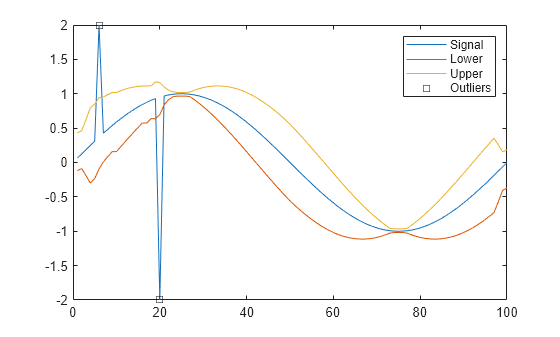
Generate 100 samples of a sinusoidal signal. Replace the sixth and twentieth samples with spikes.
x = sin(2*pi*(0:99)/100);
x(6) = 2;
x(20) = -2;
Use hampel to locate every sample that differs by more than three standard deviations from the local median. The measurement window is composed of the sample and its six surrounding samples, three per side.
[y,i,xmedian,xsigma] = hampel(x);
Plot the filtered signal and annotate the outliers.
n = 1:length(x);
plot(n,x)
hold on
plot(n,xmedian-3*xsigma,n,xmedian+3*xsigma)
plot(find(i),x(i),'sk')
hold off
legend('Original signal','Lower limit','Upper limit','Outliers')

Repeat the computation, but now take just one adjacent sample on each side when computing the median. The function considers the extrema as outliers.
hampel(x,1)

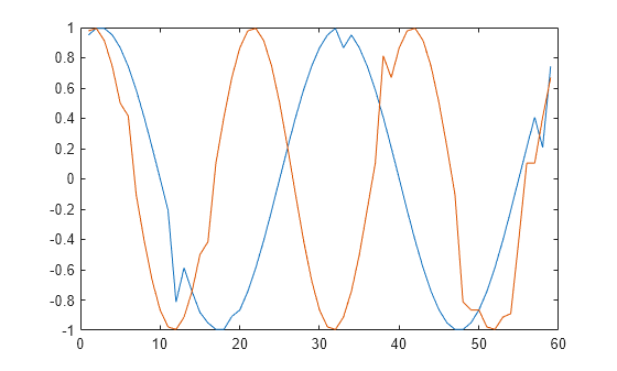
Generate a two-channel signal consisting of sinusoids of different frequencies. Place spikes in random places. Use NaNs to add missing samples at random. Reset the random number generator for reproducible results. Plot the signal.
rng('default')

n = 59;
x = sin(pi./[15 10]'*(1:n)+pi/3)';

spk = randi(2*n,9,1);
x(spk) = x(spk)*2;
x(randi(2*n,6,1)) = NaN;

plot(x)
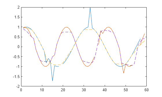
Filter the signal using hampel with the default settings.
y = hampel(x);
plot(y)

Increase the length of the moving window and decrease the threshold to treat a sample as an outlier.
y = hampel(x,4,2);
plot(y)
Output the running median for each channel. Overlay the medians on a plot of the signal.
[y,j,xmd,xsd] = hampel(x,4,2);
plot(x)
hold on
plot(xmd,'--')
Generate a multichannel signal that consists of two sinusoids of different frequencies embedded in white Gaussian noise of unit variance.
rng('default')

t = 0:60;
x = sin(pi./[10;2]*t)'+randn(numel(t),2);
Apply a Hampel filter to the signal. Take as outliers those points that differ by more than two standard deviations from the median of a surrounding nine-sample window. Output a logical matrix that is true at the locations of the outliers.
k = 4;
nsig = 2;

[y,h] = hampel(x,k,nsig);
Plot each channel of the signal in its own set of axes. Draw the original signal, the filtered signal, and the outliers. Annotate the outlier locations.
for k = 1:2
    hk = h(:,k);
    ax = subplot(2,1,k);
    plot(t,x(:,k))
    hold on
    plot(t,y(:,k))
    plot(t(hk),x(hk,k),'*')
    hold off
    ax.XTick = t(hk);
end
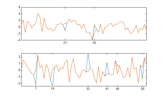
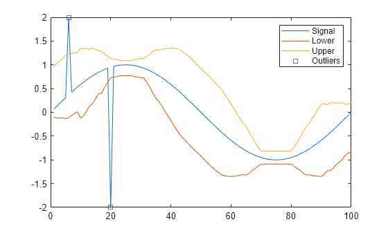
Generate 100 samples of a sinusoidal signal. Replace the sixth and twentieth samples with spikes.
n = 1:100;
x = sin(2*pi*n/100);
x(6) = 2;
x(20) = -2;
Use hampel to compute the local median and estimated standard deviation for every sample. Use the default values of the input parameters:
The window size is .
The points that differ from their window median by more than three standard deviations are considered outliers.
Plot the result.
[y,i,xmedian,xsigma] = hampel(x);

plot(n,x)
hold on
plot(n,[1;1]*xmedian+3*[-1;1]*xsigma)
plot(find(i),x(i),'sk')
hold off
legend('Signal','Lower','Upper','Outliers')
Repeat the calculation using a window size of and two standard deviations as the criteria for identifying outliers.
sds = 2;
adj = 10;
[y,i,xmedian,xsigma] = hampel(x,adj,sds);

plot(n,x)
hold on
plot(n,[1;1]*xmedian+sds*[-1;1]*xsigma)
plot(find(i),x(i),'sk')
hold off
legend('Signal','Lower','Upper','Outliers')
Input Arguments
Output Arguments
More About
References
[1] Liu, Hancong, Sirish Shah, and Wei Jiang. "On-line outlier detection and data cleaning." Computers and Chemical Engineering. Vol. 28, March 2004, pp. 1635–1647.
[2] Suomela, Jukka. "Median Filtering Is Equivalent to Sorting." https://arxiv.org/pdf/1406.1717, 2014.
Extended Capabilities
Version History
Introduced in R2015b
See Also
medfilt1 | median | filloutliers | filter | isoutlier | mad (Statistics and Machine Learning Toolbox) | movmad | movmedian | sgolayfilt