Optimize Satellite Link Budget to Maximize Bit Rate
This example shows how to optimize the satellite link budget to maximize the bit rate. In this example, you tune the link budget parameters to maximize the achievable bit rate for a given link margin by optimizing the transmitter high-power amplifier (HPA) power, transmitter antenna diameter, and receiver gain-to-noise temperature ratio (G/T). The optimization is subject to the constraints on transmitter effective isotropic radiated power (EIRP), received power, and antenna gain.
This example requires the Optimize Live Editor task from the Optimization Toolbox™.
Baseline Link Budget Using Exported Script
To generate the baseline link budget, this example uses the default MATLAB® script exported from the Satellite Link Budget Analyzer app. The app can analyze uplink (L1), downlink (L2), and crosslink (L3). This example considers only uplink optimization, but you can extend the same concepts to other links. To generate the equivalent MATLAB script from the Satellite Link Budget Analyzer app, on the app toolstrip, click Export.
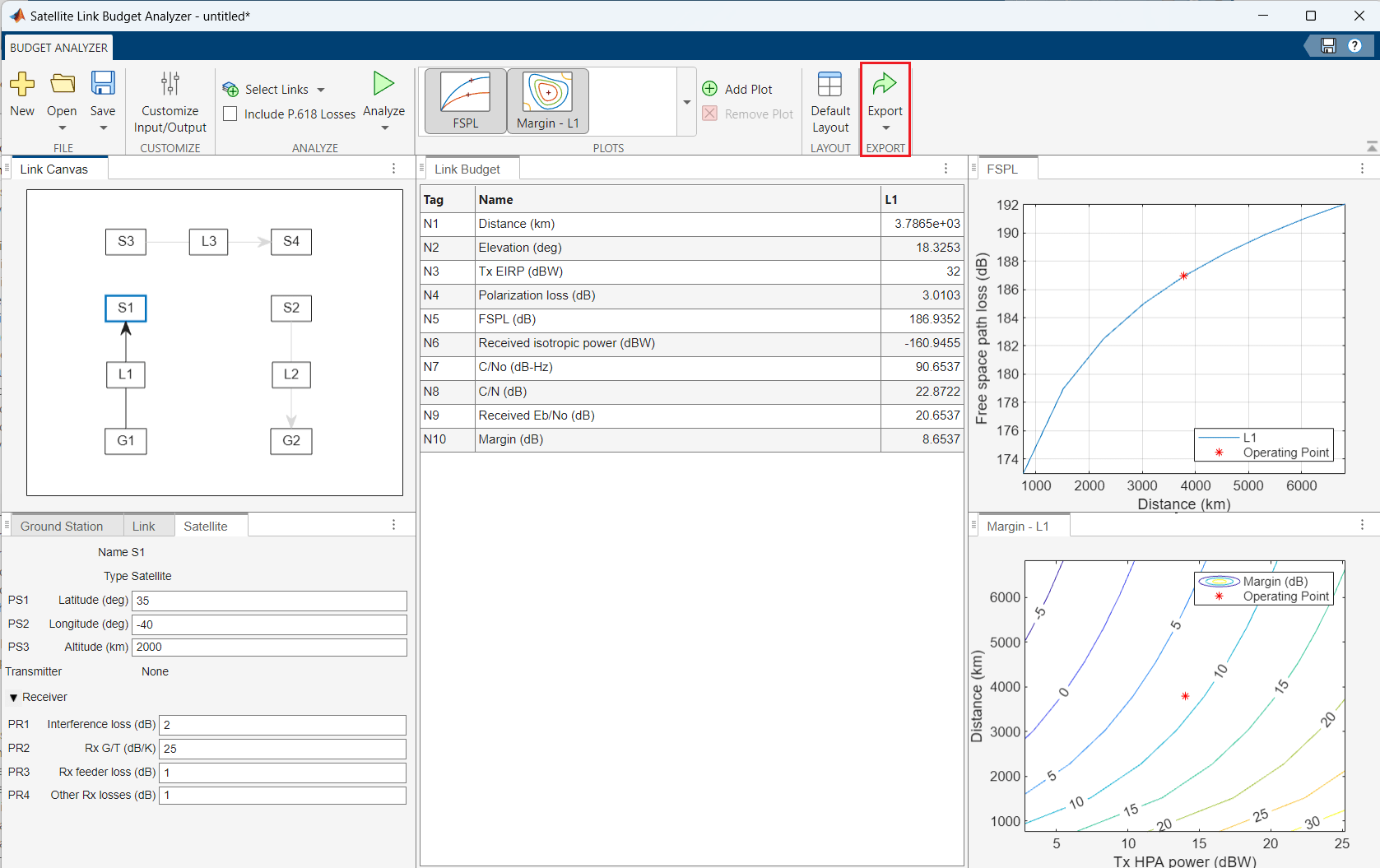
This figure shows part of the script generated by the Satellite Link Budget Analyzer app.

By default, the app exports these properties for the link (L1), ground station (G1), and satellite (S1).
%% Satellite (S1) properties
s1.Latitude = 35;              % deg
s1.Longitude = -40;            % deg
s1.Altitude = 2000;            % km

%% Satellite (S1) receiver properties
rx1.InterferenceLoss = 2;      % dB
rx1.RxGByT = 25;               % dB/K
rx1.RxFeederLoss = 1;          % dB
rx1.OtherRxLosses = 1;         % dB

%% Link (L1) properties
l1.Frequency = 14;             % GHz
l1.Bandwidth = 6;              % MHz
l1.BitRate = 10;               % Mbps
l1.RequiredEbByNo = 10;        % dB
l1.PolarizationMismatch = 45;  % deg
l1.ImplementationLoss = 2;     % dB
l1.AntennaMispointingLoss = 1; % dB
l1.RadomeLoss = 1;             % dB

%% Ground station (G1) location properties
g1.Latitude = 42.3;            % deg
g1.Longitude = -71.35;         % deg
g1.Altitude = 20;              % m

%% Ground station (G1) transmitter properties
tx1.TxFeederLoss = 2;          % dB
tx1.OtherTxLosses = 3;         % dB
tx1.TxHPAPower = 14;           % dBW
tx1.TxHPAOBO = 6;              % dB
tx1.TxAntennaGain = 30;        % dBi
Compute the baseline link margin by using the local function calculateLinkBudget with the default satellite, ground station, link, transmitter, and receiver values from the exported script.
resultsBaseline = calculateLinkBudget(g1,s1,tx1,rx1,l1)
resultsBaseline = struct with fields:
                  Distance: 3.7865e+03
                 Elevation: 18.3253
                    TxEIRP: 32
          PolarizationLoss: 3.0103
                      FSPL: 186.9352
    ReceivedIsotropicPower: -160.9455
                     CByNo: 90.6537
                      CByN: 22.8722
            ReceivedEbByNo: 20.6537
                    Margin: 8.6537
Additional Link Budget Parameters
Define the additional link budget parameters to use in optimization. This example assumes a transmitter antenna efficiency of 0.6, a noise temperature of 200 K, and a link margin of 3 dB.
txAntennaEfficiency = 0.6;
noiseTemperature = 200;    % K
linkMargin = 3;            % dB
Estimate the received Eb/No required to achieve a particular bit error rate (BER) by using the RequiredEbByNo and ImplementationLoss properties of L1 and the specified link margin.
receivedEbByNo = l1.RequiredEbByNo + l1.ImplementationLoss + linkMargin; % dBSet Up and Solve Optimization Problem
The optimization problem in this example aims to create an objective function that maximizes the bit rate, in Mbps, for a given link margin. The problem uses these design variables and constraints:
Design variables – Transmitter HPA power, transmitter antenna diameter, and receiver G/T
Constraints – Transmitter EIRP, antenna gain, and received power
Set Design Variables
Tune the optimization variables: the transmitter antenna diameter, representing a parabolic dish, the HPA output power, and the receiver G/T. To reduce the search space, specify bounds on the optimization variables. In this example, HPA power must be in the range [10, 20] dBW, antenna diameter must be in the range [0.5, 4.5] m, and receiver G/T must be in the range [10, 20] dB/K.
minHPAPower = 10;           % dBW
maxHPAPower = 20;           % dBW
minTxAntennaDiameter = 0.5; % m
maxTxAntennaDiameter = 4.5; % m
minRxGByT = 10;             % dB/K
maxRxGByT = 20;             % dB/K
Set Constraints of the Optimization Goal
The design must also satisfy constraints for minimum received power, maximum antenna gain, and maximum transmitter EIRP. Define limits on antenna gain, received power, and transmitter EIRP. These limits apply to the constraints part of the optimization problem.
maxAntennaGain = 40;    % dB
minReceivedPower = -95; % dBm
maxTxEIRP = 40;         % dB
Build and Solve Optimization Problem
To build and solve the problem, use the Optimize Live Editor task. You can add the Optimize Live Editor task into the script by, on the Live Editor or Insert tab of the MATLAB toolstrip, selecting Task > Optimize.
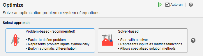
Select Problem-based. For more information on the problem-based Optimize Live Editor task, see Get Started with Problem-Based Optimize Live Editor Task (Optimization Toolbox).
This task has already been populated with the design variables, objective function, and constraints.
% Create optimization variables
hpaPowerDB2 = optimvar("hpaPowerDB","LowerBound",minHPAPower,"UpperBound",...
    maxHPAPower);
rxGByT2 = optimvar("rxGByT","LowerBound",minRxGByT,"UpperBound",maxRxGByT);
antennaDiameter2 = optimvar("antennaDiameter","LowerBound",...
    minTxAntennaDiameter,"UpperBound",maxTxAntennaDiameter);

% Set initial starting point for the solver
initialPoint.hpaPowerDB = minHPAPower;
initialPoint.rxGByT = minRxGByT;
initialPoint.antennaDiameter = minTxAntennaDiameter;

% Create problem
problem = optimproblem("ObjectiveSense","Maximize");

% Define problem objective
problem.Objective = fcn2optimexpr(@objectiveFcn,hpaPowerDB2,rxGByT2,...
    antennaDiameter2,txAntennaEfficiency,receivedEbByNo,g1,s1,tx1,rx1,l1);

% Define problem constraints
problem.Constraints.constraint1 = rxGByT2 + 10.*(log(noiseTemperature)/log(10)) <= maxAntennaGain;
problem.Constraints.constraint2 = gainCalc(antennaDiameter2,...
    txAntennaEfficiency,l1.Frequency) <= maxAntennaGain;
problem.Constraints.constraint3 = receiverSensitivityConstraint(hpaPowerDB2,...
    rxGByT2,antennaDiameter2,noiseTemperature,txAntennaEfficiency,...
    minReceivedPower,g1,s1,tx1,rx1,l1);
problem.Constraints.constraint4 = txEIRPConstraint(hpaPowerDB2,...
    antennaDiameter2,txAntennaEfficiency,maxTxEIRP,g1,s1,tx1,rx1,l1);

% Display problem information
show(problem);
  OptimizationProblem :

	Solve for:
       antennaDiameter, hpaPowerDB, rxGByT

	maximize :
       arg1

       where:

           arg1 = objectiveFcn(hpaPowerDB, rxGByT, antennaDiameter, 0.6, 15, extraParams{1}, extraParams{2}, extraParams{3}, extraParams{4}, extraParams{5});

       extraParams


	subject to constraint1:
       rxGByT <= 16.9897

	subject to constraint2:
       (10 .* (log((0.6 .* ((3.1416 .* antennaDiameter) ./ 0.021414).^2)) ./ 2.3026)) <= 40

	subject to constraint3:
       arg_LHS >= (-95)

       where:

             arg1 = ((((((((hpaPowerDB - 6) - 2) - 3) + (10 .* (log((0.6 .* ((3.1416 .* antennaDiameter) ./ 0.021414).^2)) ./ 2.3026))) - 1) - 3.0103) - 186.9352) - 2);
             arg_LHS = (((((arg1 - 1) + rxGByT) + 23.0103) - 1) + 30);

	subject to constraint4:
       (((((hpaPowerDB - 6) - 2) - 3) + (10 .* (log((0.6 .* ((3.1416 .* antennaDiameter) ./ 0.021414).^2)) ./ 2.3026))) - 1) <= 40

	variable bounds:
       0.5 <= antennaDiameter <= 4.5

       10 <= hpaPowerDB <= 20

       10 <= rxGByT <= 20
% Solve problem
[solution2,objectiveValue,reasonSolverStopped] = solve(problem,initialPoint);
Solving problem using fmincon. Local minimum found that satisfies the constraints. Optimization completed because the objective function is non-decreasing in feasible directions, to within the value of the optimality tolerance, and constraints are satisfied to within the value of the constraint tolerance. <stopping criteria details>
% Display results
solution2
solution2 = struct with fields:
antennaDiameter: 0.8202
hpaPowerDB: 12.6108
rxGByT: 16.9897
reasonSolverStopped
reasonSolverStopped =
    OptimalSolution
objectiveValue
objectiveValue =
3.6673e+07
% Clear variables
clearvars hpaPowerDB2 rxGByT2 antennaDiameter2 initialPoint reasonSolverStopped...
    objectiveValue
Analyze Results
Compare the design parameters and metrics for the baseline and optimized designs. The optimized design increases the final bit rate to over 36 Mbps, but trades off HPA power, antenna diameter, and G/T. Also, observe that the design achieves the specified link margin.
uit = analyzeResults(solution2,resultsBaseline,g1,s1,tx1,rx1,l1,txAntennaEfficiency,noiseTemperature,receivedEbByNo);

Further Exploration
This example maximizes bit rate by using optimization capabilities in a MATLAB script generated from the Satellite Link Budget Analyzer app. Try running this example with these modifications.
Change the link margins and observe the bit rate.
Consider different objective functions, design variables, and constraints.
Consider additional physical, cost, or manufacturing constraints.
References
[1] Berrezzoug, S., F. T. Bendimerad, and A. Boudjemai. “Communication Satellite Link Budget Optimization Using Gravitational Search Algorithm.” In 2015 3rd International Conference on Control, Engineering & Information Technology (CEIT), 1–7. Tlemcen, Algeria: IEEE, 2015. https://doi.org/10.1109/CEIT.2015.7233120.
[2] Cheung, K. “The Role of Margin in Link Design and Optimization.” In 2015 IEEE Aerospace Conference, 1–11. Big Sky, MT: IEEE, 2015. https://doi.org/10.1109/AERO.2015.7119220.
Local Functions
receiverSensitivityConstraint – Constraint for minimum received power.
function constraint = receiverSensitivityConstraint(hpaPowerDBParam,rxGByTParam,antennaDiameterParam,noiseTemperature,txAntennaEfficiency,minReceivedPower,gs,sat,tx,rx,link)

rxdPower = fcn2optimexpr(@receiverSensitivity,hpaPowerDBParam,rxGByTParam,antennaDiameterParam,noiseTemperature,gs,sat,tx,rx,link,txAntennaEfficiency);
constraint = rxdPower >= minReceivedPower;
end

function rxdPower = receiverSensitivity(hpaPowerDBParam,rxGByTParam,antennaDiameterParam,noiseTemperature,gs,sat,tx,rx,link,txAntennaEfficiency)

tx.TxHPAPower = hpaPowerDBParam;
rx.RxGByT = rxGByTParam;
tx.TxAntennaGain = gainCalc(antennaDiameterParam,txAntennaEfficiency,link.Frequency);
res = calculateLinkBudget(gs,sat,tx,rx,link);
rxdPower = res.ReceivedIsotropicPower + rx.RxGByT + 10.*(log(noiseTemperature)/log(10)) - rx.RxFeederLoss + 30;                                        % dBm

end
txEIRPConstraint – Constraint for maximum transmitter EIRP.
function constraint = txEIRPConstraint(hpaPowerDBParam,antennaDiameterParam,txAntennaEfficiency,maxTxEIRP,gs,sat,tx,rx,link)

eirp = fcn2optimexpr(@txEIRP,hpaPowerDBParam,antennaDiameterParam,gs,sat,tx,rx,link,txAntennaEfficiency);
constraint = eirp <= maxTxEIRP;
end

function eirp = txEIRP(hpaPowerDBParam,antennaDiameterParam,gs,sat,tx,rx,link,txAntennaEfficiency)

tx.TxHPAPower = hpaPowerDBParam;
tx.TxAntennaGain = gainCalc(antennaDiameterParam,txAntennaEfficiency,link.Frequency);
res = calculateLinkBudget(gs,sat,tx,rx,link);
eirp = res.TxEIRP;

end
objectiveFcn – Objective function for maximizing the bit rate.
function bitRate = objectiveFcn(hpaPowerDBParam,rxGByTParam,antennaDiameterParam,txAntennaEfficiency,receivedEbByNo,gs,sat,tx,rx,link)

tx.TxHPAPower = hpaPowerDBParam;
rx.RxGByT = rxGByTParam;
tx.TxAntennaGain = gainCalc(antennaDiameterParam,txAntennaEfficiency,link.Frequency);
res = calculateLinkBudget(gs,sat,tx,rx,link);
bitRateDB = res.CByNo - receivedEbByNo;
bitRate = 10.^(bitRateDB/10);

end
gainCalc – Calculate gain for parabolic antenna.
function gdB = gainCalc(antennaDiameterParam,antennaEfficiency,freq)
lambda = physconst('LightSpeed')/(freq*1e9);                         % Frequency in GHz
g = antennaEfficiency*(pi*antennaDiameterParam/lambda).^2;
gdB = 10.*(log(g)/log(10));
end
calculateLinkBudget – Calculate the link budget result parameters.
function res = calculateLinkBudget(spec,sat,tx,rx,lnk,varargin)
assignin("base","struct1",spec);
assignin("base","struct2",sat);
assignin("base","struct3",tx);
assignin("base","struct4",rx);
assignin("base","struct5",lnk);
resultProperty = [];
resultVariable = [];
if nargin > 5
    resultVariable = varargin{1};
end
if nargin == 8
    resultProperty = varargin{2};
    resultValue = varargin{3};
end
params = {"Distance"; "Elevation"; "TxEIRP"; "PolarizationLoss"; ...
    "FSPL"; "ReceivedIsotropicPower"; "CByNo"; "CByN"; ...
    "ReceivedEbByNo"; "Margin"};
eqns = {"satcom.internal.linkbudgetApp.computeDistance(struct1.Latitude, struct1.Longitude, struct1.Altitude, struct2.Latitude, struct2.Longitude, struct2.Altitude*1e3)"; ...
    "satcom.internal.linkbudgetApp.computeElevation(struct1.Latitude, struct1.Longitude, struct1.Altitude, struct2.Latitude, struct2.Longitude, struct2.Altitude*1e3)"; ...
    "struct3.TxHPAPower - struct3.TxHPAOBO - struct3.TxFeederLoss - struct3.OtherTxLosses + struct3.TxAntennaGain - struct5.RadomeLoss"; ...
    "20 * abs(log10(cosd(struct5.PolarizationMismatch)))"; ...
    "fspl(temp.Distance * 1e3, physconst('LightSpeed') ./ (struct5.Frequency*1e9))"; ...
    "temp.TxEIRP - temp.PolarizationLoss - temp.FSPL - struct4.InterferenceLoss - struct5.AntennaMispointingLoss"; ...
    "temp.ReceivedIsotropicPower + struct4.RxGByT - 10*log10(physconst('Boltzmann')) - struct4.RxFeederLoss - struct4.OtherRxLosses"; ...
    "temp.CByNo - 10*log10(struct5.Bandwidth) - 60"; ...
    "temp.CByNo - 10*log10(struct5.BitRate) - 60"; ...
    "temp.ReceivedEbByNo - struct5.RequiredEbByNo - struct5.ImplementationLoss"};
if nargin == 7
    vectorSpecValue = varargin{2};
    eqns{1} = mat2str(vectorSpecValue);
end
for ii = 1:length(params)
    varname = strcat("temp.",params{ii});
    if any(strcmp(resultProperty,params{ii}))
        evalin("base",sprintf("%s = %f;",varname,resultValue(strcmp(resultProperty,params{ii}))))
    else
        evalin("base",sprintf("%s = %s;",varname,eqns{ii}))
    end
    if strcmp(resultVariable,params{ii}) && ~isempty(resultVariable)
        break;
    end
end
res = evalin("base","temp");
evalin("base","clear struct1 struct2 struct3 struct4 struct5 temp")
end
analyzeResults – Analyze and visualize the optimization results.
function uit = analyzeResults(sol,resBaseline,g1,s1,tx1,rx1,l1,txAntennaEfficiency,noiseTemperature,receivedEbByNo)

gainBaselineLinear = 10.^(tx1.TxAntennaGain/10);
lambda = physconst('LightSpeed')/(l1.Frequency*1e9);
txAntennaDiameterBaseline = sqrt(gainBaselineLinear/txAntennaEfficiency)*(lambda/pi);
receivedPowerBaseline = resBaseline.ReceivedIsotropicPower + rx1.RxGByT + 10.*(log(noiseTemperature)/log(10)) - rx1.RxFeederLoss + 30; %dBm
dataBefore = [struct2cell(resBaseline); {tx1.TxHPAPower;...
    txAntennaDiameterBaseline; tx1.TxAntennaGain; rx1.RxGByT; receivedPowerBaseline; l1.BitRate}];

tx1.TxHPAPower = sol.hpaPowerDB;
rx1.RxGByT = sol.rxGByT;
tx1.TxAntennaGain = gainCalc(sol.antennaDiameter,txAntennaEfficiency,l1.Frequency);
res = calculateLinkBudget(g1,s1,tx1,rx1,l1);
res.ReceivedEbByNo = receivedEbByNo;
res.Margin = res.ReceivedEbByNo - l1.RequiredEbByNo - l1.ImplementationLoss;
receivedPower = res.ReceivedIsotropicPower + rx1.RxGByT + 10.*(log(noiseTemperature)/log(10)) - rx1.RxFeederLoss + 30;                %dBm
bitRate = 10.^((res.CByNo - res.ReceivedEbByNo)/10);
dataAfter = [struct2cell(res); {sol.hpaPowerDB; ...
    sol.antennaDiameter; tx1.TxAntennaGain; sol.rxGByT; receivedPower; 1e-6*bitRate}];

colName = {"Link Before","Link After"};
colFormat = {'numeric','numeric'};
rowNames = { ...
    "Distance (km)";
    "Elevation (deg)";
    "Tx EIRP (dBW)";
    "Polarization loss (dB)";
    "FSPL (dB)";
    "Received isotropic power (dBW)";
    "C/No (dB-Hz)";
    "C/N (dB)";
    "Received Eb/No (dB)";
    "Margin (dB)";
    "HPA Power (dBW)";
    "Tx Antenna Diameter (m)";
    "Tx Antenna Gain (dBi)";
    "Rx G/T (dB/K)";
    "Received Power (dBm)";
    "Bit Rate (Mbps)"};
fig = uifigure("Name","Link Budget");
uit = uitable(fig,units="normalized", ...
    Position=[0 0 1 1],RowName=rowNames, ...
    ColumnName=colName, ColumnFormat=colFormat, ...
    Data=[dataBefore dataAfter]);
style = uistyle(BackgroundColor="yellow",FontColor="k",FontWeight="bold");
addStyle(uit,style,"row",[3 7 11:16])
end