Get Started with Problem-Based Optimize Live Editor Task

This example script helps you to use the problem-based Optimize Live Editor task for optimization or equation solving. Modify the script for your own problem.

The script solves a nonlinear optimization problem with nonlinear constraints:

Minimize $$rosenbrock(x,y,a)=\log (1+a(y-x^2{)}^2+(1-x{)}^2)$$ subject to the constraint $$x^2+y^2\le 1$$, where $$a=100$$ and the initial point $$x0$$ has $$x=-2,y=2$$. Also, impose the bounds $$-3\le x\le 3$$, $$-2\le y\le 9$$.

The code for the objective function appears at the end of this script.

Include Parameters or Data

Typically, you have data or values to pass to the solver. Place those values in the input section (where you see x0x and x0y) and run the section by choosing Section > Run Section or pressing Control+Enter.

Set the initial point components x0x and x0y and scale a for the optimization.

x0x = -2;
x0y = 2;
a = 100;

Place these values and any other problem data into the workspace by running this section before proceeding.

Optimize Live Editor Task

Usually, you place the Optimize Live Editor task into the script by selecting Task > Optimize in the Live Editor tab, or by selecting Task > Optimize in the Insert tab. Then you are presented with the following choice (this is only a picture, not the real task):

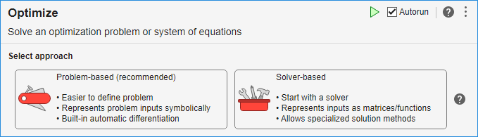
To get the problem-based task, click Problem-based (recommended).

The following problem-based task has the variables, objective, and constraint filled in. Modify it for your problem, or run it as is to see how the task works. To modify the problem, click the Define problem button at the bottom of the task. To run the task, click the Solve problem button at the bottom of the task.

  OptimizationProblem : 

	Solve for:
       x, y

	minimize :
       log(((1 + (100 .* (y - x.^2).^2)) + (1 - x).^2))


	subject to :
       (x.^2 + y.^2) <= 1

	variable bounds:
       -3 <= x <= 3

       -2 <= y <= 9

Solving problem using fmincon.

Local minimum found that satisfies the constraints.

Optimization completed because the objective function is non-decreasing in 
feasible directions, to within the value of the optimality tolerance,
and constraints are satisfied to within the value of the constraint tolerance.

solution = struct with fields:
    x: 0.7864
    y: 0.6177

reasonSolverStopped = 
    OptimalSolution

objectiveValue = 0.0447

Interpret Results

The task calls solve, which calls fmincon to solve the problem. The top of the task shows that the solution is returned in the solution structure. The reported solution, x = 0.7864 and y = 0.6177, satisfies the constraint $$x^2+y^2\le 1$$, as you can see in the following calculation.

solution.x^2 + solution.y^2                                     

ans = 1.0000

The solver reports exit condition OptimalSolution when it stops. To interpret this condition, look at the exitflag Output Arguments for the fmincon solver. The description states "First-order optimality measure is less than options.OptimalityTolerance, and maximum constraint violation is less than options.ConstraintTolerance." In other words, the solution is a feasible local minimum.

The objective function value at the solution is 0.0457. This is the smallest objective function value among feasible points.

Helper Functions

This code creates the rosenbrock helper function.

function objective = rosenbrock(x,y,a)
% This function should return a scalar representing an optimization objective.

% Example: Concession stand profit
% revenue = 3*soda + 5*popcorn + 2*candy;
% cost = 1*soda + 2*popcorn + 0.75*candy;
% objective = revenue - cost; % profit

% Edit the lines below with your calculations.
objective = log(1 + a*(y - x^2)^2 + (1 - x)^2);
end