Control of Aircraft Lateral Axis Using Mu Synthesis
This example shows how to use mu-analysis and synthesis tools in the Robust Control Toolbox™. It describes the design of a robust controller for the lateral-directional axis of an aircraft during powered approach to landing. The linearized model of the aircraft is obtained for an angle-of-attack of 10.5 degrees and airspeed of 140 knots.
Performance Specifications
The illustration below shows a block diagram of the closed-loop system. The diagram includes the nominal aircraft model, the controller K, as well as elements capturing the model uncertainty and performance objectives (see next sections for details).
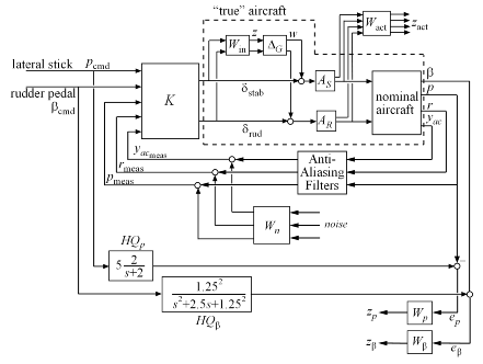
Figure 1: Robust Control Design for Aircraft Lateral Axis
The design goal is to make the airplane respond effectively to the pilot's lateral stick and rudder pedal inputs. The performance specifications include:
Decoupled responses from lateral stick
p_cmdto roll ratepand from rudder pedalsbeta_cmdto side-slip anglebeta. The lateral stick and rudder pedals have a maximum deflection of +/- 1 inch.The aircraft handling quality (HQ) response from lateral stick to roll rate
pshould match the first-order response.
HQ_p    = 5.0 * tf(2.0,[1 2.0]);
step(HQ_p), title('Desired response from lateral stick to roll rate (Handling Quality)')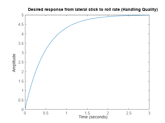
Figure 2: Desired response from lateral stick to roll rate.
The aircraft handling quality response from the rudder pedals to the side-slip angle
betashould match the damped second-order response.
HQ_beta = -2.5 * tf(1.25^2,[1 2.5 1.25^2]);
step(HQ_beta), title('Desired response from rudder pedal to side-slip angle (Handling Quality)')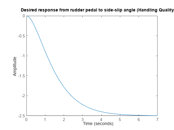
Figure 3: Desired response from rudder pedal to side-slip angle.
The stabilizer actuators have +/- 20 deg and +/- 50 deg/s limits on their deflection angle and deflection rate. The rudder actuators have +/- 30 deg and +/-60 deg/s deflection angle and rate limits.
The three measurement signals ( roll rate
p, yaw rater, and lateral accelerationyac) are filtered through second-order anti-aliasing filters:
freq = 12.5 * (2*pi);  % 12.5 Hz
zeta = 0.5;
yaw_filt = tf(freq^2,[1 2*zeta*freq freq^2]);
lat_filt = tf(freq^2,[1 2*zeta*freq freq^2]);

freq = 4.1 * (2*pi);  % 4.1 Hz
zeta = 0.7;
roll_filt = tf(freq^2,[1 2*zeta*freq freq^2]);

AAFilters = append(roll_filt,yaw_filt,lat_filt);
From Specs to Weighting Functions
H-infinity design algorithms seek to minimize the largest closed-loop gain across frequency (H-infinity norm). To apply these tools, we must first recast the design specifications as constraints on the closed-loop gains. We use weighting functions to "normalize" the specifications across frequency and to equally weight each requirement.
We can express the design specs in terms of weighting functions as follows:
To capture the limits on the actuator deflection magnitude and rate, pick a diagonal, constant weight
W_act, corresponding to the stabilizer and rudder deflection rate and deflection angle limits.
W_act = ss(diag([1/50,1/20,1/60,1/30]));
Use a 3x3 diagonal, high-pass filter
W_nto model the frequency content of the sensor noise in the roll rate, yaw rate, and lateral acceleration channels.
W_n = append(0.025,tf(0.0125*[1 1],[1 100]),0.025);
clf, bodemag(W_n(2,2)), title('Sensor noise power as a function of frequency')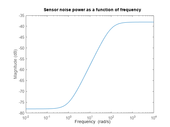
Figure 4: Sensor noise power as a function of frequency
The response from lateral stick to
pand from rudder pedal tobetashould match the handling quality targetsHQ_pandHQ_beta. This is a model-matching objective: to minimize the difference (peak gain) between the desired and actual closed-loop transfer functions. Performance is limited due to a right-half plane zero in the model at 0.002 rad/s, so accurate tracking of sinusoids below 0.002 rad/s is not possible. Accordingly, we'll weight the first handling quality spec with a bandpass filterW_pthat emphasizes the frequency range between 0.06 and 30 rad/sec.
W_p = tf([0.05 2.9 105.93 6.17 0.16],[1 9.19 30.80 18.83 3.95]);
clf, bodemag(W_p), title('Weight on Handling Quality spec')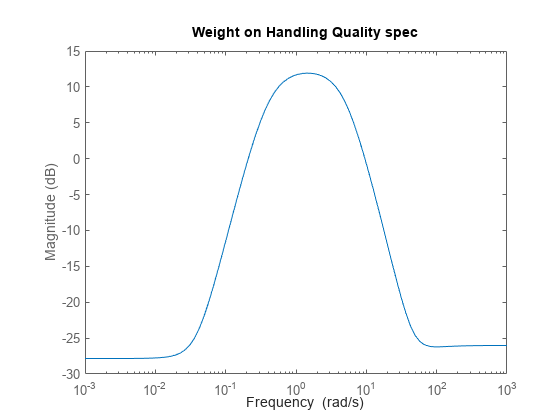
Figure 5: Weight on handling quality spec.
Similarly, pick
W_beta=2*W_pfor the second handling quality spec
W_beta = 2*W_p;
Here we scaled the weights W_act, W_n, W_p, and W_beta so the closed-loop gain between all external inputs and all weighted outputs is less than 1 at all frequencies.
Nominal Aircraft Model
A pilot can command the lateral-directional response of the aircraft with the lateral stick and rudder pedals. The aircraft has the following characteristics:
Two control inputs: differential stabilizer deflection
delta_stabin degrees, and rudder deflectiondelta_rudin degrees.Three measured outputs: roll rate
pin deg/s, yaw raterin deg/s, and lateral accelerationyacin g's.One calculated output: side-slip angle
beta.
The nominal lateral directional model LateralAxis has four states:
Lateral velocity
vYaw rate
rRoll rate
pRoll angle
phi
These variables are related by the state space equations:
where x = [v; r; p; phi], u = [delta_stab; delta_rud], and y = [beta; p; r; yac].
load LateralAxisModel
LateralAxis
LateralAxis =
A =
v r p phi
v -0.116 -227.3 43.02 31.63
r 0.00265 -0.259 -0.1445 0
p -0.02114 0.6703 -1.365 0
phi 0 0.1853 1 0
B =
delta_stab delta_rud
v 0.0622 0.1013
r -0.005252 -0.01121
p -0.04666 0.003644
phi 0 0
C =
v r p phi
beta 0.2469 0 0 0
p 0 0 57.3 0
r 0 57.3 0 0
yac -0.002827 -0.007877 0.05106 0
D =
delta_stab delta_rud
beta 0 0
p 0 0
r 0 0
yac 0.002886 0.002273
Continuous-time state-space model.
Model Properties
The complete airframe model also includes actuators models A_S and A_R. The actuator outputs are their respective deflection rates and angles. The actuator rates are used to penalize the actuation effort.
A_S = [tf([25 0],[1 25]); tf(25,[1 25])];
A_S.OutputName = {'stab_rate','stab_angle'};

A_R = A_S;
A_R.OutputName = {'rud_rate','rud_angle'};
Accounting for Modeling Errors
The nominal model only approximates true airplane behavior. To account for unmodeled dynamics, you can introduce a relative term or multiplicative uncertainty W_in*Delta_G at the plant input, where the error dynamics Delta_G have gain less than 1 across frequencies, and the weighting function W_in reflects the frequency ranges in which the model is more or less accurate. There are typically more modeling errors at high frequencies so W_in is high pass.
% Normalized error dynamics
Delta_G = ultidyn('Delta_G',[2 2],'Bound',1.0);

% Frequency shaping of error dynamics
w_1 = tf(2.0*[1 4],[1 160]);
w_2 = tf(1.5*[1 20],[1 200]);
W_in = append(w_1,w_2);

bodemag(w_1,'-',w_2,'--')
title('Relative error on nominal model as a function of frequency')
legend('stabilizer','rudder','Location','NorthWest');
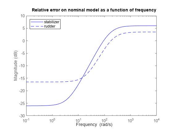
Figure 6: Relative error on nominal aircraft model as a function of frequency.
Building an Uncertain Model of the Aircraft Dynamics
Now that we have quantified modeling errors, we can build an uncertain model of the aircraft dynamics corresponding to the dashed box in the Figure 7 (same as Figure 1):

Figure 7: Aircraft dynamics.
Use the connect function to combine the nominal airframe model LateralAxis, the actuator models A_S and A_R, and the modeling error description W_in*Delta_G into a single uncertain model Plant_unc mapping [delta_stab; delta_rud] to the actuator and plant outputs:
% Actuator model with modeling uncertainty
Act_unc = append(A_S,A_R) * (eye(2) + W_in*Delta_G);
Act_unc.InputName = {'delta_stab','delta_rud'};

% Nominal aircraft dynamics
Plant_nom = LateralAxis;
Plant_nom.InputName = {'stab_angle','rud_angle'};

% Connect the two subsystems
Inputs = {'delta_stab','delta_rud'};
Outputs = [A_S.y ; A_R.y ; Plant_nom.y];
Plant_unc = connect(Plant_nom,Act_unc,Inputs,Outputs);
This produces an uncertain state-space (USS) model Plant_unc of the aircraft:
Plant_unc
Uncertain continuous-time state-space model with 8 outputs, 2 inputs, 8 states.
The model uncertainty consists of the following blocks:
  Delta_G: Uncertain 2x2 LTI, peak gain = 1, 1 occurrences
Model Properties

Type "Plant_unc.NominalValue" to see the nominal value and "Plant_unc.Uncertainty" to interact with the uncertain elements.
Analyzing How Modeling Errors Affect Open-Loop Responses
We can analyze the effect of modeling uncertainty by picking random samples of the unmodeled dynamics Delta_G and plotting the nominal and perturbed time responses (Monte Carlo analysis). For example, for the differential stabilizer channel, the uncertainty weight w_1 implies a 5% modeling error at low frequency, increasing to 100% after 93 rad/sec, as confirmed by the Bode diagram below.
% Pick 10 random samples
Plant_unc_sampl = usample(Plant_unc,10);

% Look at response from differential stabilizer to beta
figure('Position',[100,100,560,500])
subplot(211), step(Plant_unc.Nominal(5,1),'r+',Plant_unc_sampl(5,1),'b-',10)
legend('Nominal','Perturbed')

subplot(212), bodemag(Plant_unc.Nominal(5,1),'r+',Plant_unc_sampl(5,1),'b-',{0.001,1e3})
legend('Nominal','Perturbed')
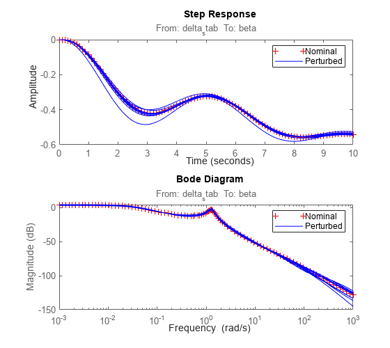
Figure 8: Step response and Bode diagram.
Designing the Lateral-Axis Controller
Proceed with designing a controller that robustly achieves the specifications, where robustly means for any perturbed aircraft model consistent with the modeling error bounds W_in.
First we build an open-loop model OLIC mapping the external input signals to the performance-related outputs as shown below.
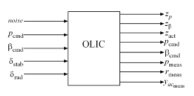
Figure 9: Open-loop model mapping external input signals to performance-related outputs.
To build this model, start with the block diagram of the closed-loop system, remove the controller block K, and use connect to compute the desired model. As before, the connectivity is specified by labeling the inputs and outputs of each block.
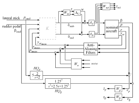
Figure 10: Block diagram for building open-loop model.
% Label block I/Os
AAFilters.u = {'p','r','yac'};    AAFilters.y = 'AAFilt';
W_n.u = 'noise';                  W_n.y = 'Wn';
HQ_p.u = 'p_cmd';                 HQ_p.y = 'HQ_p';
HQ_beta.u = 'beta_cmd';           HQ_beta.y = 'HQ_beta';
W_p.u = 'e_p';                    W_p.y = 'z_p';
W_beta.u = 'e_beta';              W_beta.y = 'z_beta';
W_act.u = [A_S.y ; A_R.y];        W_act.y = 'z_act';

% Specify summing junctions
Sum1 = sumblk('%meas = AAFilt + Wn',{'p_meas','r_meas','yac_meas'});
Sum2 = sumblk('e_p = HQ_p - p');
Sum3 = sumblk('e_beta = HQ_beta - beta');

% Connect everything
OLIC = connect(Plant_unc,AAFilters,W_n,HQ_p,HQ_beta,...
   W_p,W_beta,W_act,Sum1,Sum2,Sum3,...
   {'noise','p_cmd','beta_cmd','delta_stab','delta_rud'},...
   {'z_p','z_beta','z_act','p_cmd','beta_cmd','p_meas','r_meas','yac_meas'});
This produces the uncertain state-space model
OLIC
Uncertain continuous-time state-space model with 11 outputs, 7 inputs, 26 states.
The model uncertainty consists of the following blocks:
  Delta_G: Uncertain 2x2 LTI, peak gain = 1, 1 occurrences
Model Properties

Type "OLIC.NominalValue" to see the nominal value and "OLIC.Uncertainty" to interact with the uncertain elements.
Recall that by construction of the weighting functions, a controller meets the specs whenever the closed-loop gain is less than 1 at all frequencies and for all I/O directions. First design an H-infinity controller that minimizes the closed-loop gain for the nominal aircraft model:
nmeas = 5;		% number of measurements
nctrls = 2;		% number of controls
[kinf,~,gamma_inf] = hinfsyn(OLIC.NominalValue,nmeas,nctrls);
gamma_inf
gamma_inf =
0.9700
Here hinfsyn computed a controller kinf that keeps the closed-loop gain below 1 so the specs can be met for the nominal aircraft model.
Next, perform a mu-synthesis to see if the specs can be met robustly when taking into account the modeling errors (uncertainty Delta_G). Use the command musyn to perform the synthesis and use musynOptions to set the frequency grid used for mu-analysis.
fmu = logspace(-2,2,60);
opt = musynOptions('FrequencyGrid',fmu);
[kmu,CLperf] = musyn(OLIC,nmeas,nctrls,opt);
D-K ITERATION SUMMARY:
-----------------------------------------------------------------
Robust performance Fit order
-----------------------------------------------------------------
Iter K Step Peak MU D Fit D
1 5.097 3.487 3.488 12
2 1.31 1.292 1.312 20
3 1.243 1.242 1.692 12
4 1.692 1.543 1.544 16
5 1.223 1.223 1.55 12
6 1.533 1.464 1.465 20
7 1.293 1.292 1.307 12
Best achieved robust performance: 1.22
CLperf
CLperf =
1.2227
Here the best controller kmu cannot keep the closed-loop gain below 1 for the specified model uncertainty, indicating that the specs can be nearly but not fully met for the family of aircraft models under consideration.
Frequency-Domain Comparison of Controllers
Compare the performance and robustness of the H-infinity controller kinf and mu controller kmu. Recall that the performance specs are achieved when the closed loop gain is less than 1 for every frequency. Use the lft function to close the loop around each controller:
clinf = lft(OLIC,kinf);
clmu = lft(OLIC,kmu);
What is the worst-case performance (in terms of closed-loop gain) of each controller for modeling errors bounded by W_in? The wcgain command helps you answer this difficult question directly without need for extensive gridding and simulation.
% Compute worst-case gain as a function of frequency
opt = wcOptions('VaryFrequency','on');

% Compute worst-case gain (as a function of frequency) for kinf
[mginf,wcuinf,infoinf] = wcgain(clinf,opt);

% Compute worst-case gain for kmu
[mgmu,wcumu,infomu] = wcgain(clmu,opt);
You can now compare the nominal and worst-case performance for each controller:
clf
subplot(211)
f = infoinf.Frequency;
gnom = sigma(clinf.NominalValue,f);
semilogx(f,gnom(1,:),'r',f,infoinf.Bounds(:,2),'b');
title('Performance analysis for kinf')
xlabel('Frequency (rad/sec)')
ylabel('Closed-loop gain');
xlim([1e-2 1e2])
legend('Nominal Plant','Worst-Case','Location','NorthWest');

subplot(212)
f = infomu.Frequency;
gnom = sigma(clmu.NominalValue,f);
semilogx(f,gnom(1,:),'r',f,infomu.Bounds(:,2),'b');
title('Performance analysis for kmu')
xlabel('Frequency (rad/sec)')
ylabel('Closed-loop gain');
xlim([1e-2 1e2])
legend('Nominal Plant','Worst-Case','Location','SouthWest');
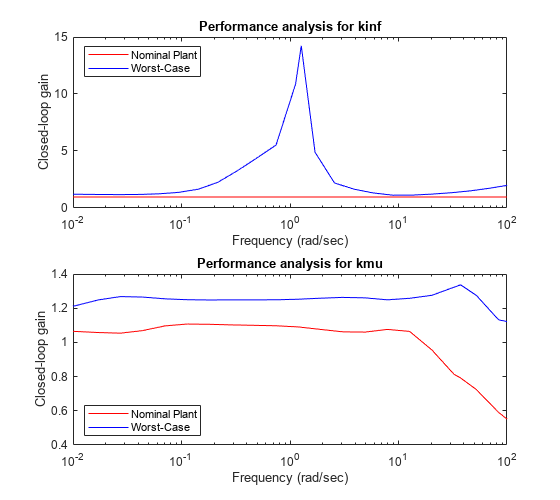
The first plot shows that while the H-infinity controller kinf meets the performance specs for the nominal plant model, its performance can sharply deteriorate (peak gain near 15) for some perturbed model within our modeling error bounds.
In contrast, the mu controller kmu has slightly worse performance for the nominal plant when compared to kinf, but it maintains this performance consistently for all perturbed models (worst-case gain near 1.25). The mu controller is therefore more robust to modeling errors.
Time-Domain Validation of the Robust Controller
To further test the robustness of the mu controller kmu in the time domain, you can compare the time responses of the nominal and worst-case closed-loop models with the ideal "Handling Quality" response. To do this, first construct the "true" closed-loop model CLSIM where all weighting functions and HQ reference models have been removed:
kmu.u = {'p_cmd','beta_cmd','p_meas','r_meas','yac_meas'};
kmu.y = {'delta_stab','delta_rud'};

AAFilters.y = {'p_meas','r_meas','yac_meas'};

CLSIM = connect(Plant_unc(5:end,:),AAFilters,kmu,{'p_cmd','beta_cmd'},{'p','beta'});
Next, create the test signals u_stick and u_pedal shown below
time = 0:0.02:15;
u_stick = (time>=9 & time<12);
u_pedal = (time>=1 & time<4) - (time>=4 & time<7);

clf
subplot(211), plot(time,u_stick), axis([0 14 -2 2]), title('Lateral stick command')
subplot(212), plot(time,u_pedal), axis([0 14 -2 2]), title('Rudder pedal command')
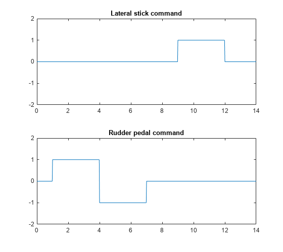
You can now compute and plot the ideal, nominal, and worst-case responses to the test commands u_stick and u_pedal.
% Ideal behavior
IdealResp = append(HQ_p,HQ_beta);
IdealResp.y = {'p','beta'};

% Worst-case response
WCResp = usubs(CLSIM,wcumu);

% Compare responses
clf
lsim(IdealResp,'g',CLSIM.NominalValue,'r',WCResp,'b:',[u_stick ; u_pedal],time)
legend('ideal','nominal','perturbed','Location','SouthEast');
title('Closed-loop responses with mu controller KMU')

The closed-loop response is nearly identical for the nominal and worst-case closed-loop systems. Note that the roll-rate response of the aircraft tracks the roll-rate command well initially and then departs from this command. This is due to a right-half plane zero in the aircraft model at 0.024 rad/sec.