diskmargin

Disk-based stability margins of feedback loops

Syntax

[DM,MM] = diskmargin(L)

MMIO = diskmargin(P,C)

___ = diskmargin(___,sigma)

Description

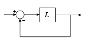
[DM,MM] = diskmargin(L) computes the disk-based stability margins for the SISO or MIMO negative feedback loop feedback(L,eye(N)), where N is the number of inputs and outputs in L.

The diskmargin command returns loop-at-a-time stability margins in DM and multiloop margins in MM. Disk-based margin analysis provides a stronger guarantee of stability than the classical gain and phase margins. For general information about disk margins, see Stability Analysis Using Disk Margins.

MMIO = diskmargin(P,C) computes the stability margins when considering independent, concurrent variations at both the plant inputs and plant outputs the negative feedback loop of the following diagram.

___ = diskmargin(___,sigma) specifies an additional skew parameter that biases the modeled gain and phase variation toward gain increase (positive sigma) or gain decrease (negative sigma). You can use this argument to test the relative sensitivity of stability margins to gain increases versus decreases. You can use this argument with any of the previous syntaxes.

Examples

Disk Margins of MIMO Feedback Loop

diskmargin computes both loop-at-a-time and multiloop disk margins. This example illustrates that loop-at-a-time margins can give an overly optimistic assessment of the true robustness of MIMO feedback loops. Margins of individual loops can be sensitive to small perturbations in other loops, and loop-at-a-time margins ignore such loop interactions.

Consider the two-channel MIMO feedback loop of the following illustration.

The plant model P is drawn from MIMO Stability Margins for Spinning Satellite and C is the static output-feedback gain [1 -2;0 1].

a = [0 10;-10 0]; 
b = eye(2); 
c = [1 10;-10 1]; 
P = ss(a,b,c,0); 
C = [1 -2;0 1]; 

Compute the disk-based margins at the plant output. The negative-feedback open-loop response at the plant output is Lo = P*C.

Lo = P*C;
[DMo,MMo] = diskmargin(Lo);

Examine the loop-at-a-time disk margins returned in the structure array DM. Each entry in DM contains the stability margins of the corresponding feedback channel.

DMo(1)

ans = struct with fields:
           GainMargin: [0 Inf]
          PhaseMargin: [-90 90]
           DiskMargin: 2
           LowerBound: 2
           UpperBound: 2
            Frequency: Inf
    WorstPerturbation: [2×2 ss]

DMo(2)

ans = struct with fields:
           GainMargin: [0 Inf]
          PhaseMargin: [-90 90]
           DiskMargin: 2
           LowerBound: 2
           UpperBound: 2
            Frequency: 0
    WorstPerturbation: [2×2 ss]

The loop-at-a-time margins are excellent (infinite gain margin and 90° phase margin). Next examine the multiloop disk margins MMo. These consider independent and concurrent gain (phase) variations in both feedback loops. This is a more realistic assessment because plant uncertainty typically affects both channels simultaneously.

MMo

MMo = struct with fields:
           GainMargin: [0.6839 1.4621]
          PhaseMargin: [-21.2607 21.2607]
           DiskMargin: 0.3754
           LowerBound: 0.3754
           UpperBound: 0.3762
            Frequency: 0
    WorstPerturbation: [2×2 ss]

The multiloop gain and phase margins are much weaker than their loop-at-a-time counterparts. Stability is only guaranteed when the gain in each loop varies by a factor less than 1.46, or when the phase of each loop varies by less than 21°. Use diskmarginplot to visualize the gain and phase margins as a function of frequency.

diskmarginplot(Lo)

Typically, there is uncertainty in both the actuators (inputs) and sensors (outputs). Therefore, it is a good idea to compute the disk margins at the plant inputs as well as the outputs. Use Li = C*P to compute the margins at the plant inputs. For this system, the margins are the same at the plant inputs and outputs.

Li = C*P;
[DMi,MMi] = diskmargin(Li);
MMi

MMi = struct with fields:
           GainMargin: [0.6839 1.4621]
          PhaseMargin: [-21.2607 21.2607]
           DiskMargin: 0.3754
           LowerBound: 0.3754
           UpperBound: 0.3762
            Frequency: 0
    WorstPerturbation: [2×2 ss]

Finally, you can also compute the multiloop disk margins for gain or phase variations at both the inputs and outputs of the plant. This approach is the most thorough assessment of stability margins, because it this considers independent and concurrent gain or phase variations in all input and output channels. As expected, of all three measures, this gives the smallest gain and phase margins.

MMio = diskmargin(P,C);
diskmarginplot(MMio.GainMargin)

Stability is only guaranteed when the gain varies by a less than 2 dB or when the phase varies by less than 13°. However, these variations take place at the inputs and the outputs of P, so the total change in I/O gain or phase is twice that.

Sensitivity of Disk-Based Margins to Gain Increase and Decrease

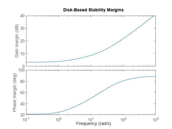
By default, diskmargin computes a symmetric gain margin, with gmin = 1/gmax, and an associated phase margin. In some systems, however, loop stability may be more sensitive to increases or decreases in open-loop gain. Use the skew parameter sigma to examine this sensitivity.

Compute the disk margin and associated disk-based gain and phase margins for a SISO transfer function, at three values of sigma. Negative sigma biases the computation toward gain decrease. Positive sigma biases toward gain increase.

L = tf(25,[1 10 10 10]);
DMdec = diskmargin(L,-2);
DMbal = diskmargin(L,0);
DMinc = diskmargin(L,2); 
DGMdec = DMdec.GainMargin

DGMdec = 1×2

    0.4013    1.3745

DGMbal = DMbal.GainMargin

DGMbal = 1×2

    0.6273    1.5942

DGMinc = DMinc.GainMargin  

DGMinc = 1×2

    0.7717    1.7247

Put together, these results show that in the absence of phase variation, stability is maintained for relative gain variations between 0.4 and 1.72. To see how the phase margin depends on these gain variations, plot the stable ranges of gain and phase variations for each diskmargin result.

diskmarginplot([DGMdec;DGMbal;DGMinc])
legend('sigma = -2','sigma = 0','sigma = 2')
title('Stable range of gain and phase variations')

This plot shows that the feedback loop can tolerate larger phase variations when the gain decreases. In other words, the loop stability is more sensitive to gain increase. Although sigma = –2 yields a phase margin as large as 30 degrees, this large value assumes a small gain increase of less than 3 dB. However, the plot shows that when the gain increases by 4 dB, the phase margin drops to less than 15 degrees. By contrast, it remains greater than 30 degrees when the gain decreases by 4 dB.

Thus, varying the skew sigma can give a fuller picture of sensitivity to gain and phase uncertainty. Unless you are mostly concerned with gain variations in one direction (increase or decrease), it is not recommended to draw conclusions from a single nonzero value of sigma. Instead use the default sigma = 0 to get unbiased estimates of gain and phase margins. When using nonzero values of sigma, use both positive and negative values to compare relative sensitivity to gain increase and decrease.

Input Arguments

L — Open-loop response

dynamic system model | model array

Open-loop response, specified as a dynamic system model. L can be SISO or MIMO, as long as it has the same number of inputs and outputs. diskmargin computes the disk-based stability margins for the negative-feedback closed-loop system feedback(L,eye(N)).

To compute the disk margins of the positive feedback system feedback(L,eye(N),+1), use diskmargin(-L).

When you have a plant P and a controller C, you can compute the disk margins for gain (or phase) variations at the plant inputs or outputs, as in the following diagram.

• To compute margins at the plant outputs, set L = P*C.

• To compute margins at the plant inputs, set L = C*P.

L can be continuous time or discrete time. If L is a generalized state-space model (genss or uss) then diskmargin uses the current or nominal value of all control design blocks in L.

If L is a frequency-response data model (such as frd), then diskmargin computes the margins at each frequency represented in the model. The function returns the margins at the frequency with the smallest disk margin.

If L is a model array, then diskmargin computes margins for each model in the array.

P — Plant

dynamic system model

Plant, specified as a dynamic system model. P can be SISO or MIMO, as long as P*C has the same number of inputs and outputs. diskmargin computes the disk-based stability margins for a negative-feedback closed-loop system. To compute the disk margins of the system with positive feedback, use diskmargin(P,-C).

P can be continuous time or discrete time. If P is a generalized state-space model (genss or uss) then diskmargin uses the current or nominal value of all control design blocks in P.

If P is a frequency-response data model (such as frd), then diskmargin computes the margins at each frequency represented in the model. The function returns the margins at the frequency with the smallest disk margin.

C — Controller

dynamic system model

Controller, specified as a dynamic system model. C can be SISO or MIMO, as long as P*C has the same number of inputs and outputs. diskmargin computes the disk-based stability margins for a negative-feedback closed-loop system. To compute the disk margins of the system with positive feedback, use diskmargin(P,-C).

C can be continuous time or discrete time. If C is a generalized state-space model (genss or uss) then diskmargin uses the current or nominal value of all control design blocks in C.

If C is a frequency-response data model (such as frd), then diskmargin computes the margins at each frequency represented in the model. The function returns the margins at the frequency with the smallest disk margin.

sigma — Skew

0 (default) | real scalar

Skew of uncertainty region used to compute the stability margins, specified as a real scalar value. This parameter biases the uncertainty used to model gain and phase variations toward gain increase or gain decrease.

• The default sigma = 0 uses a balanced model of gain variation in a range [gmin,gmax], with gmin = 1/gmax.

• Positive sigma uses a model with more gain increase than decrease (gmax > 1/gmin).

• Negative sigma uses a model with more gain decrease than increase (gmin < 1/gmax).

Use the default sigma = 0 to get unbiased estimates of gain and phase margins. You can test relative sensitivity to gain increase and decrease by comparing the margins obtained with both positive and negative sigma values. For an example, see Sensitivity of Disk-Based Margins to Gain Increase and Decrease. For more detailed information about how the choice of sigma affects the margin computation, see Stability Analysis Using Disk Margins.

Output Arguments

DM — Disk margins for each feedback channel

structure | structure array

Disk margins for each feedback channel with all other loops closed, returned as a structure for SISO feedback loops, or an N-by-1 structure array for a MIMO loop with N feedback channels. The fields of DM(i) are:

Field	Value
GainMargin	Disk-based gain margins of the corresponding feedback channel, returned as a vector of the form [gmin,gmax]. These values express in absolute units the amount by which the loop gain in that channel can decrease or increase while preserving stability. For example, if DM(i).GainMargin = [0.8,1.25] then the gain of the ith loop can be multiplied by any factor between 0.8 and 1.25 without causing instability. When sigma = 0, gmin = 1/gmax. If the open-loop gain can change sign without loss of stability, gmin can be less than zero for large enough negative sigma. If the nominal closed-loop system is unstable, then DM(i).GainMargin = [1 1].
PhaseMargin	Disk-based phase margin of the corresponding feedback channel, returned as a vector of the form [-pm,pm] in degrees. These values express the amount by which the loop phase in that channel can decrease or increase while preserving stability. If the closed-loop system is unstable, then DM(i).PhaseMargin = [0 0].
DiskMargin	Maximum ɑ compatible with closed-loop stability for the corresponding feedback channel. ɑ parameterizes the uncertainty in the loop response (see Algorithms). If the closed-loop system is unstable, then DM(i).DiskMargin = 0.
LowerBound	Lower bound on disk margin. This value is the same as DiskMargin.
UpperBound	Upper bound on disk margin. This value represents an upper limit on the actual disk margin of the system. In other words, the disk margin is guaranteed to be no worse than LowerBound and no better than UpperBound.
Frequency	Frequency at which the weakest margin occurs for the corresponding loop channel. This value is in rad/TimeUnit, where TimeUnit is the TimeUnit property of L.
WorstPerturbation	Smallest gain and phase variation that drives the feedback loop unstable, returned as a state-space (ss) model with N inputs and outputs, where N is the number of inputs and outputs in L. The system F(s) = WorstPerturbation is such that the following feedback loop is marginally stable, with a pole on the stability boundary at the frequency DM(i).Frequency. This state-space model is a diagonal perturbation of the form F(s) = diag(f1(s),...,fN(s)). Each fj(s) is a real-parameter dynamic system that realizes the worst-case complex gain and phase variation applied to each channel of the feedback loop. For the loop-at-a-time margin of the kth feedback loop, only the kth entry fk(s) of DM(k).WorstPerturbation differs from unity. For more information on interpreting WorstPerturbation, see Disk Margin and Smallest Destabilizing Perturbation. When analyzing a linear approximation of a nonlinear system, it can be useful to inject WorstPerturbation into the nonlinear simulation to further analyze the destabilizing affect of this worst-case gain and phase variation. For an example, see Robust MIMO Controller for Two-Loop Autopilot.

When L = P*C is the open-loop response of a system comprising a controller and plant with unit negative feedback in each channel, DM contains the stability margins for variations at the plant outputs. To compute the stability margins for variations at the plant inputs, use L = C*P. To compute the stability margins for simultaneous, independent variations at both the plant inputs and outputs, use MMIO = diskmargin(P,C).

When L is a model array, DM has additional dimensions corresponding to the array dimensions of L. For instance, if L is a 1-by-3 array of two-input, two-output models, then DM is a 2-by-3 structure array. DM(j,k) contains the margins for the j^th feedback channel of the k^th model in the array.

MM — Multiloop disk margins

structure

Multiloop disk margins, returned as a structure. The gain (or phase) margins quantify how much gain variation (or phase variation) the system can tolerate in all feedback channels at once while remaining stable. Thus, MM is a single structure regardless of the number of feedback channels in the system. (For SISO systems, MM = DM.) The fields of MM are:

Field	Value
GainMargin	Multiloop disk-based gain margins, returned as a vector of the form [gmin,gmax]. These values express in absolute units the amount by which the loop gain can vary in all channels independently and concurrently while preserving stability. For example, if MM.GainMargin = [0.8,1.25] then the gain of all loops can be multiplied by any factor between 0.8 and 1.25 without causing instability. When sigma = 0, gmin = 1/gmax.
PhaseMargin	Multiloop disk-based phase margin, returned as a vector of the form [-pm,pm] in degrees. These values express the amount by which the loop phase can vary in all channels independently and concurrently while preserving stability.
DiskMargin	Maximum ɑ compatible with closed-loop stability. ɑ parameterizes the uncertainty in the loop response (see Algorithms).
LowerBound	Lower bound on disk margin. This value is the same as DiskMargin.
UpperBound	Upper bound on disk margin. This value represents an upper limit on the actual disk margin of the system. In other words, the disk margin is guaranteed to be no worse than LowerBound and no better than UpperBound.
Frequency	Frequency at which the weakest margin occurs. This value is in rad/TimeUnit, where TimeUnit is the TimeUnit property of L.
WorstPerturbation	Smallest gain and phase variation that drives the feedback loop unstable, returned as a state-space (ss) model with N inputs and outputs, where N is the number of inputs and outputs in L. The system F(s) = WorstPerturbation is such that the following feedback loop is marginally stable, with a pole on the stability boundary at MM.Frequency. This state-space model is a diagonal perturbation of the form F(s) = diag(f1(s),...,fN(s)). Each fj(s) is a real-parameter dynamic system that realizes the worst-case complex gain and phase variation applied to each channel of the feedback loop. For more information on interpreting WorstPerturbation, see Disk Margin and Smallest Destabilizing Perturbation When analyzing a linear approximation of a nonlinear system, it can be useful to inject WorstPerturbation into the nonlinear simulation to further analyze the destabilizing affect of this worst-case gain and phase variation. For an example, see Robust MIMO Controller for Two-Loop Autopilot.

When L = P*C is the open-loop response of a system comprising a controller and plant with unit negative feedback in each channel, MM contains the stability margins for variations at the plant outputs. To compute the stability margins for variations at the plant inputs, use L = C*P. To compute the stability margins for simultaneous, independent variations at both the plant inputs and outputs, use MMIO = diskmargin(P,C).

When L is a model array, MM is a structure array with one entry for each model in L.

MMIO — Disk margins for independent variations in all input and output channels

structure

Disk margins for independent variations applied simultaneously at input and output channels of the plant P, returned as a structure having the same fields as MM.

For variations applied simultaneously at inputs and outputs, the WorstPerturbation field is itself a structure with fields Input and Output. Each of these fields contains a state-space model such that for Fi(s) = MMIO.WorstPerturbation.Input and Fo(s) = MMIO.WorstPerturbation.Output, the system of the following diagram is marginally unstable, with a pole on the stability boundary at the frequency MMIO.Frequency.

These state-space models Input and Output are diagonal perturbations of the form F(s) = diag(f1(s),...,fN(s)). Each fj(s) is a real-parameter dynamic system that realizes the worst-case complex gain and phase variation applied to each channel of the feedback loop.

Tips

• diskmargin assumes negative feedback. To compute the disk margins of a positive feedback system, use diskmargin(-L) or diskmargin(P,-C).

• To compute disk margins for a system modeled in Simulink^®, first linearize the model to obtain the open-loop response at a particular operating point. Then, use diskmargin to compute stability margins for the linearized system. For more information, see Stability Margins of a Simulink Model.

• To compute classical gain and phase margins, use allmargin.

• You can visualize disk margins using diskmarginplot.

Algorithms

diskmargin computes gain and phase margins by applying a disk-based uncertainty model to represent gain and phase variations, and then finding the largest such disk for which the closed-loop system is stable.

Gain and Phase Uncertainty Model

For SISO L, the uncertainty model for disk-margin analysis incorporates a multiplicative complex uncertainty F into the loop transfer function as follows:

$$F=\frac{1+\alpha \left[\left(1-\sigma \right)/2\right]\delta }{1-\alpha \left[\left(1+\sigma \right)/2\right]\delta }.$$

Here,

• δ is a gain-bounded dynamic uncertainty, normalized so that it always varies within the unit disk (|δ| < 1).

• α sets the amount of gain and phase variation modeled by F. For fixed σ, the parameter ɑ controls the size of the disk. For α = 0, the multiplicative factor is 1, corresponding to the nominal L.

• σ, called the skew, biases the modeled uncertainty toward gain increase or gain decrease. (For details about the effect of skew on the uncertainty model, see Stability Analysis Using Disk Margins.)

For MIMO systems, the model allows the uncertainty to vary independently in each channel:

$$F_j=\frac{1+\alpha \left[\left(1-\sigma \right)/2\right]{\delta }_j}{1-\alpha \left[\left(1+\sigma \right)/2\right]{\delta }_j}.$$

The model replaces the MIMO open-loop response L with L*F, where

$$F=\left(\begin{array}{ccc}{F}_1& 0& 0\\ 0& \ddots & 0\\ 0& 0& F_N\end{array}\right).$$

Disk-Margin Computation

For a given value of the skew sigma, the disk margin is the largest ɑ for which the closed-loop system feedback(L*F,1) (or feedback(L*F,eye(N)) for MIMO systems) is stable for all values of F. To find this value, diskmargin solves a robust stability problem: Find the largest α such that the closed-loop system is stable for all F in the uncertainty disk Δ(α,σ) described by

$$\Delta \left(\alpha ,\sigma \right)=\left\{F=\frac{1+\alpha \left[\left(1-\sigma \right)/2\right]\delta }{1-\alpha \left[\left(1+\sigma \right)/2\right]\delta }:\left|\delta \right|<1\right\}.$$

In the SISO case, the robust stability analysis leads to

$${\alpha }_{max}=\frac{1}{{\Vert S+\left(\sigma -1\right)/2\Vert }_{\infty }},$$

where S is the sensitivity function (1 + L)^–1 .

In the MIMO case, the robust stability analysis leads to

$${\alpha }_{max}=\frac{1}{{\mu }_{\Delta }\left(S+\frac{\left(\sigma -1\right)I}{2}\right)}.$$

Here, μ_Δ is the structured singular value (mussv) for the diagonal structure

$$\Delta =\left(\begin{array}{ccc}{\delta }_1& 0& 0\\ 0& \ddots & 0\\ 0& 0& {\delta }_N\end{array}\right),$$

and δ_j is the normalized uncertainty for each F_j.

For more details about the margin computation, see [2].

References

[1] Blight, James D., R. Lane Dailey, and Dagfinn Gangsaas. “Practical Control Law Design for Aircraft Using Multivariable Techniques.” International Journal of Control 59, no. 1 (January 1994): 93–137. https://doi.org/10.1080/00207179408923071.

[2] Seiler, Peter, Andrew Packard, and Pascal Gahinet. “An Introduction to Disk Margins [Lecture Notes].” IEEE Control Systems Magazine 40, no. 5 (October 2020): 78–95.

Version History

Introduced in R2018b

R2020a: Obtain smallest destabilizing gain or phase perturbations

diskmargin now returns the smallest gain and phase variations that drive the feedback loop unstable in the WorstPerturbation field of the output structures DM, MM, and MMIO.

R2020a: Disk-based gain-margin range can include negative gains

diskmargin returns disk-based gain margins in the GainMargin field of its output structures DM, MM, and MMIO. These margins take the form [gmin,gmax], meaning that the open-loop gain can be multiplied by any factor in that range without loss of closed-loop stability. Beginning in R2020a, the lower end of the range gmin can be negative for some negative values of the skew sigma, if the closed-loop system remains stable even if the sign of the open-loop gain changes. The skew controls the bias in the disk-based gain margin toward gain decrease or increase (see Stability Analysis Using Disk Margins). Previously, the gain-margin range was always positive.

R2019a: Obtain lower and upper bounds on true disk margin

The algorithm used by diskmargin involves a μ structured singular-value computation that produces lower and upper estimates on the true disk margin. The output structures DM, MM, and MMIO now include fields LowerBound and UpperBound containing these bounds.