Stability Margins of a Simulink Model

This example illustrates how to compute classical and disk-based gain and phase margins of a control loop modeled in Simulink®. To compute stability margins, linearize the model to extract the open-loop responses at one or more operating points of interest. Then, use allmargin or diskmargin to compute the classical or disk-based stability margins, respectively.

MIMO Control Loop

For this example, use the Simulink model airframemarginEx.slx. This model is based on the example Trim and Linearize an Airframe (Simulink Control Design).

open_system('airframemarginEx.slx')

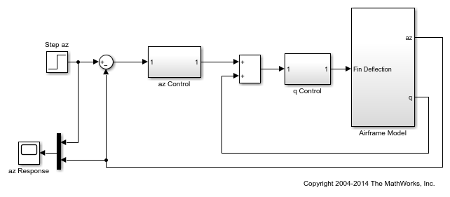
The system is a two-channel feedback loop. The plant is the one-input, two-output subsystem Airframe Model, and the controller is a two-input, one-output system whose inputs are the normal acceleration az and pitch rate q, and whose output is the Fin Deflection signal.

Loop Transfer Functions

To compute the gain margins and phase margins for this feedback system, linearize the model to get the open-loop transfer functions at the plant outputs and input. You can do so using linearization analysis points of the loop-transfer type. For more information about linearization analysis points, see Specify Portion of Model to Linearize (Simulink Control Design).

Create a loop-transfer analysis point for the plant input, which is the first output port of the q Control subsystem.

ioInput = linio('airframemarginEx/q Control',1,'looptransfer');

Similarly, create analysis points for the plant outputs. Because there are two outputs, specify these analysis points as a vector of linearization I/O objects.

ioOutput(1) = linio('airframemarginEx/Airframe Model',1,'looptransfer');
ioOutput(2) = linio('airframemarginEx/Airframe Model',2,'looptransfer');

Linearize the model to obtain the open-loop transfer functions. For this example, use the operating point specified in the model. The loop transfer at the plant input is SISO, while the loop transfer at the outputs is 2-by-2.

Li = linearize('airframemarginEx',ioInput);   % SISO
Lo = linearize('airframemarginEx',ioOutput);  % MIMO

Classical Gain and Phase Margins

To compute the classical gain margins and phase margins, use allmargin. For an open-loop transfer function, allmargin assumes a negative-feedback loop.

The open-loop transfer function returned by the linearize command is the actual linearized open-loop response of the model at the analysis point. Thus, for an open-loop response L, the closed-loop response of the entire model is a positive feedback loop.

Therefore, use -L to make allmargin compute the stability margins with positive feedback. Compute the classical gain and phase margins at the plant input.

Si = allmargin(-Li)

Si = 

  struct with fields:

     GainMargin: [0.1633 17.6557]
    GMFrequency: [1.5747 47.5259]
    PhaseMargin: 44.4560
    PMFrequency: 5.3932
    DelayMargin: 14.3866
    DMFrequency: 5.3932
         Stable: 1

The structure Si contains information about classical stability margins. For instance, Li.GMFrequency gives the two frequencies at which the phase of the open-loop response crosses –180°. Li.GainMargin gives the gain margin at each of those frequencies. The gain margin is the amount by which the loop gain can vary at that frequency while preserving closed-loop stability.

Compute the stability margins at the plant output.

So = allmargin(-Lo);

Because there are two output channels, allmargin returns an array containing one structure for each channel. Each entry contains the margins computed for that channel with the other feedback channel closed. Index into the structure So to obtain the stability margins for each channel. For instance, examine the margins with respect to gain variations or phase variations at the q output of the plant, which is the second output.

So(2)

ans = 

  struct with fields:

     GainMargin: [0.3456 17.4299]
    GMFrequency: [3.4362 49.8480]
    PhaseMargin: [-78.2447 52.6040]
    PMFrequency: [1.5685 6.5428]
    DelayMargin: [313.5198 14.0324]
    DMFrequency: [1.5685 6.5428]
         Stable: 1

Disk-Based Gain and Phase Margins

Disk margins provide a stronger guarantee of stability than the classical gain and phase margins. Disk-based margin analysis models gain and phase variations as a complex uncertainty on the open-loop system response. The disk margin is the smallest such uncertainty that is compatible with closed-loop stability. (For general information about disk margins, see Stability Analysis Using Disk Margins.)

To compute disk-based margins, use diskmargin. Like allmargin, the diskmargin command assumes a negative-feedback system. Thus, use -Li to compute the disk-based margins at the plant input.

DMi = diskmargin(-Li)

DMi = 

  struct with fields:

           GainMargin: [0.4419 2.2628]
          PhaseMargin: [-42.3153 42.3153]
           DiskMargin: 0.7740
           LowerBound: 0.7740
           UpperBound: 0.7740
            Frequency: 4.2515
    WorstPerturbation: [1x1 ss]

The field DMi.GainMargin tells you that the open-loop gain at the plant input can vary by any factor between about 0.44 and about 2.26 without loss of closed-loop stability. Disk-based margins take into account variations at all frequencies.

For a MIMO loop transfer function such as the response Lo at the plant outputs, there are two types of disk-based stability margins. The loop-at-a-time margins are the stability margins in each channel with the other loop closed. The multiloop margins are the margins for independent variations in gain (or phase) in both channels simultaneously. diskmargin computes both.

[DMo,MMo] = diskmargin(-Lo);

The loop-at-a-time margins are returned as a structure array DMo with one entry for each channel. For instance, examine the margins for gain variations or phase variations at the q output of the plant with the az loop closed, and compare with the classical margins given by So(2) above.

DMo(2)

ans = 

  struct with fields:

           GainMargin: [0.3771 2.6521]
          PhaseMargin: [-48.6811 48.6811]
           DiskMargin: 0.9047
           LowerBound: 0.9047
           UpperBound: 0.9047
            Frequency: 4.4982
    WorstPerturbation: [2x2 ss]

The multiloop margin, MMo, takes into account loop interaction by considering simultaneous variations in gain (or phase) across all feedback channels. This typically gives the most realistic stability margin estimate for multiloop control systems.

MMo

MMo = 

  struct with fields:

           GainMargin: [0.6238 1.6030]
          PhaseMargin: [-26.0867 26.0867]
           DiskMargin: 0.4633
           LowerBound: 0.4633
           UpperBound: 0.4643
            Frequency: 3.6830
    WorstPerturbation: [2x2 ss]

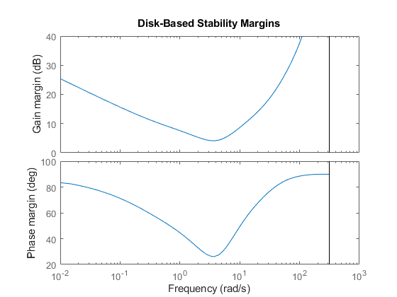
MMo.GainMargin shows that the gains in both output channels can vary independently by factors between about 0.62 and 1.60 without compromising closed-loop stability. MMo.PhaseMargin shows that stability is preserved for independent phase variations in each channel of up to ±26°. Use diskmarginplot to examine the multiloop margins graphically.

diskmarginplot(-Lo)

This shows the disk-based gain and phase margins as a function of frequency. The MMo values returned by diskmargin correspond to the weakest disk margin across frequency.

Margins at Multiple Operating Points

When you use linearize, you can provide multiple operating points to generate an array of linearizations of the system. allmargin and diskmargin can operate on linear model arrays to return the margins at multiple operating points. For example, linearize the airframe system at three simulation snapshot times.

Snap = [0; 2; 5];
LiSnap = linearize('airframemarginEx',ioInput,Snap);
LoSnap = linearize('airframemarginEx',ioOutput,Snap);

LiSnap is a 3-by-1 array of SISO linear models, one for the loop transfer at the plant input obtained at each snapshot time. Similarly, LoSnap is a 3-by-1 array of 2-input, 2-output linear models representing the loop transfers at the plant outputs at each snapshot time. Compute the classical gain and phase margins at the plant inputs at the three snapshot times.

SiSnap = allmargin(-LiSnap);

Each entry in the structure array SiSnap contains the classical margin information for the corresponding snapshot time. For instance, examine the classical margins for the second entry, t = 2 s.

SiSnap(2)

ans = 

  struct with fields:

     GainMargin: [0.0171 18.2473]
    GMFrequency: [0.0502 51.4401]
    PhaseMargin: 93.1041
    PMFrequency: 2.8474
    DelayMargin: 57.0690
    DMFrequency: 2.8474
         Stable: 1

Compute the disk margins at the plant outputs.

[DMoSnap,MMoSnap] = diskmargin(-LoSnap);

Because there are two feedback channels and three snapshot times, the structure array containing the loop-at-a-time disk margins has dimensions 2-by-3. The first dimension is for the feedback channels, and the second is for the snapshot times. In other words, DMoSnap(j,k) contains the margins for the channel j at the snapshot time k. For instance, examine the disk margins in the second feedback channel at the third snapshot time, t = 5 s.

DMoSnap(2,3)

ans = 

  struct with fields:

           GainMargin: [0.1345 7.4338]
          PhaseMargin: [-74.6771 74.6771]
           DiskMargin: 1.5257
           LowerBound: 1.5257
           UpperBound: 1.5257
            Frequency: 24.1993
    WorstPerturbation: [2x2 ss]

There is only one set of multiloop margins for each snapshot time, so MMoSnap is a 3-by-1 structure array.

As before, you can also plot the multiloop margins. There are now three curves, one for each snapshot time. Click on a curve to identify which snapshot time it corresponds to.

diskmarginplot(-LoSnap)