inverseKinematics

Create inverse kinematic solver

Description

The inverseKinematics System object™ creates an inverse kinematic (IK) solver to calculate joint configurations for a desired end-effector pose based on a specified rigid body tree model. Create a rigid body tree model for your robot using the rigidBodyTree class. This model defines all the joint constraints that the solver enforces. If a solution is possible, the joint limits specified in the robot model are obeyed.

The IK solver uses a gradient-descent-based optimization approach to find a joint configuration that is a local minimum of the weighted pose-error-squared objective function:

$$\underset{q}{\arg \min }{\Vert w\text{'}\cdot pose\_err(T_{\text{des}},FK(q,\text{ee\_link}))\Vert }_2^2,$$

where:

• w is the six-element weight vector. You can specify this using the weights argument to prioritize the relative importance between orientation and translation components.

• $$pose\_err(T_{\text{des}},FK(q,\text{ee\_link})$$ is a vector-valued function representing the six-element pose error between the desired end-effector pose T_des and the forward kinematics computed end-effector pose.

• FK is a forward kinematics function that calculates the pose at a joint configuration q for the end-effector link ee_link of the robot.

To specify more constraints besides the end-effector pose, including aiming constraints, position bounds, or orientation targets, consider using generalizedInverseKinematics. This object allows you to compute multiconstraint IK solutions.

For closed-form analytical IK solutions, see analyticalInverseKinematics.

To compute joint configurations for a desired end-effector pose:

1. Create the inverseKinematics object and set its properties.

2. Call the object with arguments, as if it were a function.

To learn more about how System objects work, see What Are System Objects?

Creation

Syntax

ik = inverseKinematics

ik = inverseKinematics(PropertyName=Value)

Description

ik = inverseKinematics creates an inverse kinematic solver. To use the solver, specify a rigid body tree model in the RigidBodyTree property.

ik = inverseKinematics(PropertyName=Value) specifies properties of the inverse kinematics solver using one or more optional name-value arguments. For example, SolverAlgorithm="fminconsqp" uses the fmincon SQP solver as the inverse kinematics solver.

Properties

Unless otherwise indicated, properties are nontunable, which means you cannot change their values after calling the object. Objects lock when you call them, and the release function unlocks them.

If a property is tunable, you can change its value at any time.

For more information on changing property values, see System Design in MATLAB Using System Objects.

RigidBodyTree — Rigid body tree model

rigidBodyTree object

Rigid body tree model, specified as a rigidBodyTree object. If you modify your rigid body tree model, reassign the rigid body tree to this property. For example:

Create IK solver and specify the rigid body tree.

ik = inverseKinematics('RigidBodyTree',rigidbodytree)

Modify the rigid body tree model.

addBody(rigidbodytree,rigidBody('body1'),'base')

Reassign the rigid body tree to the IK solver. If the solver or the step function is called before modifying the rigid body tree model, use release to allow the property to be changed.

ik.RigidBodyTree = rigidbodytree;

SolverAlgorithm — Algorithm for solving inverse kinematics

"BFGSGradientProjection" (default) | "LevenbergMarquardt" | "fminconsqp"

Algorithm for solving inverse kinematics, specified as "BFGSGradientProjection", "LevenbergMarquardt", or "fminconsqp". For details on each algorithm, see Inverse Kinematics Algorithms.

The "fminconsqp" algorithm requires Optimization Toolbox™.

SolverParameters — Parameters associated with algorithm

structure

Parameters associated with the specified algorithm, specified as a structure. The fields in the structure are specific to the algorithm. See Solver Parameters.

Usage

Syntax

[configSol,solInfo] = ik(endeffector,pose,weights,initialguess)

Description

[configSol,solInfo] = ik(endeffector,pose,weights,initialguess) finds a joint configuration that achieves the specified end-effector pose. Specify an initial guess for the configuration and your desired weights on the tolerances for the six components of pose. Solution information related to execution of the algorithm, solInfo, is returned with the joint configuration solution, configSol.

Input Arguments

endeffector — End-effector name

character vector

End-effector name, specified as a character vector. The end effector must be a frame on the rigidBodyTree object specified in the inverseKinematics System object.

pose — End-effector pose

4-by-4 homogeneous transform

End-effector pose, specified as a 4-by-4 homogeneous transform. This transform defines the desired position and orientation of the rigid body specified in the endeffector property.

weights — Weight for pose tolerances

six-element vector

Weight for pose tolerances, specified as a six-element vector. The first three elements correspond to the weights on the error in orientation for the desired pose. The last three elements correspond to the weights on the error in xyz position for the desired pose.

The solver minimizes the weighted squared norm of the pose error vector. Set weights to zero to ignore specific rotation or translation components or increase the weights to prioritize certain components. The optimization stops when this weighted error norm is less than the value of the SolutionTolerance field of the SolverParameters property.

Example: Weights vector [0,0,0,100,1,1] sets a high priority for the desired end-effector x-position in the base frame of the robot.

initialguess — Initial guess of robot configuration

structure array | vector

Initial guess of robot configuration, specified as a structure array or vector. Use this initial guess to help guide the solver to a desired robot configuration. The solution is not guaranteed to be close to this initial guess.

To use the vector form, set the DataFormat property of the object assigned in the RigidBodyTree property to either "row" or "column".

Output Arguments

configSol — Robot configuration solution

structure array | vector

Robot configuration, returned as a structure array. The structure array contains these fields:

• JointName — Character vector for the name of the joint specified in the RigidBodyTree robot model

• JointPosition — Position of the corresponding joint

This joint configuration is the computed solution that achieves the desired end-effector pose within the solution tolerance.

Note

For revolute joints, if the joint limits exceed a range of 2*pi, where joint position wrapping occurs, then the returned joint position is the one closest to the joint's lower bound.

To use the vector form, set the DataFormat property of the object assigned in the RigidBodyTree property to either "row" or "column".

solInfo — Solution information

structure

Solution information, returned as a structure. The solution information structure contains these fields:

• Iterations — Number of iterations run by the algorithm.

• NumRandomRestarts — Number of random restarts because algorithm got stuck in a local minimum.

• PoseErrorNorm — The magnitude of the pose error for the solution compared to the desired end-effector pose.

• ExitFlag — Code that gives more details on the algorithm execution and what caused it to return. For the exit flags of each algorithm type, see Exit Flags.

• Status — Character vector describing whether the solution is within the tolerance ('success') or the best possible solution the algorithm could find ('best available').

Object Functions

To use an object function, specify the System object as the first input argument. For example, to release system resources of a System object named obj, use this syntax:

release(obj)

Common to All System Objects

step	Run System object algorithm
release	Release resources and allow changes to System object property values and input characteristics
reset	Reset internal states of System object

Examples

Generate Joint Positions to Achieve End-Effector Position

Load a PUMA 560 manipulator from the Robotics System Toolbox™ loadrobot.

puma = loadrobot("puma560");

Set the desired end-effector position and convert to an SE(3) homogeneous transformation matrix.

pos = [-0.5 0.5 0.75];
eePoseTF = trvec2tform(pos);

Create the IK solver and set weights such that the solver prioritizes reaching the desired xyz-position over the desired orientation. Use the home joint configuration as the initial guess for the solver.

ik = inverseKinematics("RigidBodyTree",puma);
weights = [0 0 0 1 1 1];
initialguess = homeConfiguration(puma);

Solve IK for the end effector of the robot model, link7.

[configSoln,solnInfo] = ik("link7",eePoseTF,weights,initialguess);

Show the generated solution configuration, which now reaches the goal position.

show(puma,configSoln);
hold on
plotTransforms(pos,eul2quat([0 0 0]),FrameSize=0.3);
axis auto padded
title("End-Effector Target Position Achieved")

Note that for most IK problems, there are multiple configurations that can reach the desired pose target. Because the solver is optimization-based, the solver could approach a solution that does not actually reach the desired pose. If this occurs, the solver automatically restarts and uses a random configuration as the initial guess. This means that running the function more than once for the same pose target could yield different configurations that all reach the pose target. To avoid randomness, you can either set the random number generator seed or you can use an initial guess that is closer to the solution while also disabling AllowRandomRestart.

ik.SolverParameters.AllowRandomRestart = false

If you must find all possible solutions, use the analyticalInverseKinematics object.

Solve Inverse Kinematics Using fmincon SQP

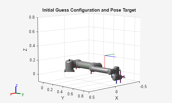
Load a robot and create an inverse kinematics solver for it. Set the solver algorithm to the fmincon SQP algorithm.

robot = loadrobot("universalUR5",DataFormat="row");
ik = inverseKinematics(RigidBodyTree=robot,SolverAlgorithm="fminconsqp");

Set the last body of the robot as the end effector, set a target pose, set the weights, and set the initial guess configuration.

ee = robot.BodyNames{end};
poseTarget = se3([0 pi/2 -pi/2],"eul","ZYX",[0 0.7 0.3]);
weights = [1 1 1 0.8 0.8 0.8];
initGuessConfig = [pi/2 0 0 0 0 0];

Show the robot in the initial guess configuration, and plot the target pose.

show(robot,initGuessConfig);
axis([-0.5 0.5 -0.1 0.9 -0.1 0.8])
hold on
plotTransforms(poseTarget,FrameSize=0.2);
title("Initial Guess Configuration and Pose Target")

Solve for a configuration that reaches the pose target using the specified weights and initial guess configuration.

[config,solninfo] = ik(ee,tform(poseTarget),weights,initGuessConfig);
show(robot,config,PreservePlot=false);
title("End-Effector Target Pose Achieved")
hold off

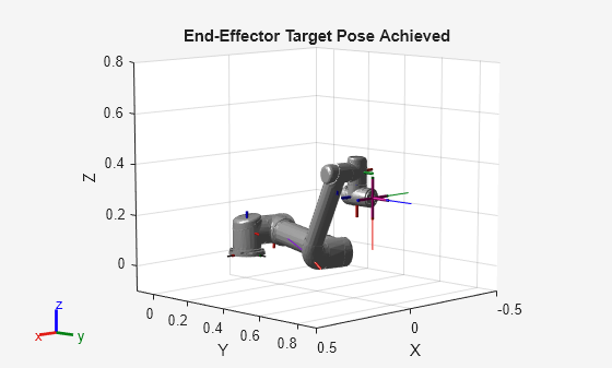
solninfo.Status

ans = 
'success'

References

[1] Badreddine, Hassan, Stefan Vandewalle, and Johan Meyers. "Sequential Quadratic Programming (SQP) for Optimal Control in Direct Numerical Simulation of Turbulent Flow." Journal of Computational Physics. 256 (2014): 1–16. doi:10.1016/j.jcp.2013.08.044.

[2] Bertsekas, Dimitri P. Nonlinear Programming. Belmont, MA: Athena Scientific, 1999.

[3] Goldfarb, Donald. "Extension of Davidon’s Variable Metric Method to Maximization Under Linear Inequality and Equality Constraints." SIAM Journal on Applied Mathematics. Vol. 17, No. 4 (1969): 739–64. doi:10.1137/0117067.

[4] Nocedal, Jorge, and Stephen Wright. Numerical Optimization. New York, NY: Springer, 2006.

[5] Sugihara, Tomomichi. "Solvability-Unconcerned Inverse Kinematics by the Levenberg–Marquardt Method." IEEE Transactions on Robotics Vol. 27, No. 5 (2011): 984–91. doi:10.1109/tro.2011.2148230.

[6] Zhao, Jianmin, and Norman I. Badler. "Inverse Kinematics Positioning Using Nonlinear Programming for Highly Articulated Figures." ACM Transactions on Graphics Vol. 13, No. 4 (1994): 313–36. doi:10.1145/195826.195827.

Extended Capabilities

C/C++ Code Generation

Generate C and C++ code using MATLAB® Coder™.

When using code generation, you must specify the RigidBodyTree property to define the robot on construction of the object. For example:

ik = inverseKinematics('RigidBodyTree',robotModel);

You also cannot change the SolverAlgorithm property after creation. To specify the solver algorithm on creation, use:

ik = inverseKinematics('RigidBodyTree',robotModel,...
        'SolverAlgorithm','LevenbergMarquardt');

Version History

Introduced in R2016b

R2026a: Specify random stream and seed for random restarts

You can use the RandomRestartParameters field of SolverParameters property to set the random stream and random number seed for random restarts. The solver uses these random restart parameters if you set the Solver parameter to either BFGS Gradient Projection or Levenberg-Marquardt, and set the AllowRandomRestarts field of the SolverParameters property to 1. For more information about the RandomRestartParameters field, see Inverse Kinematics Algorithms.

R2025a: fmincon available as IK solver algorithm

The inverseKinematics System object now supports using the fmincon SQP solver as the IK solver. See the SolverAlgorithm property for more information.

This algorithm requires Optimization Toolbox.

R2025a: Specify endeffector frame in inverseKinematics system object

You can now specify the endeffector input argument as a frame name instead of a body name in the rigid body tree.

R2019b: inverseKinematics was renamed

The inverseKinematics object was renamed from robotics.InverseKinematics. Use inverseKinematics for all object creation.