Logistic

Create Logistic model object for lifetime probability of default

Since R2020b

Description

Create and analyze a Logistic model object to calculate the lifetime probability (PD) of default using this workflow:

1. Use fitLifetimePDModel to create a Logistic model object.

2. Use predict to predict the conditional PD and predictLifetime to predict the lifetime PD.

3. Use modelDiscrimination to return AUROC and ROC data. You can plot the results using modelDiscriminationPlot.

4. Use modelCalibration to return the RMSE of the observed and predicted PD data. You can plot the results using modelCalibrationPlot.

Creation

Syntax

LogisticPDModel = fitLifetimePDModel(data,ModelType)

LogisticPDModel = fitLifetimePDModel(___,Name,Value)

Description

LogisticPDModel = fitLifetimePDModel(data,ModelType) creates a Logistic PD model object.

If you do not specify variable information for IDVar, AgeVar, LoanVars, MacroVars, and ResponseVar, then:

• IDVar is set to the first column in the data input.

• LoanVars is set to include all columns from the second to the second-to-last columns of the data input.

• ResponseVar is set to the last column in the data input.

LogisticPDModel = fitLifetimePDModel(___,Name,Value) specifies options using one or more name-value pair arguments in addition to the input arguments in the previous syntax. The optional name-value pair arguments set model object properties. For example, LogisticPDModel = fitLifetimePDModel(data(TrainDataInd,:),"Logistic",'ModelID',"Logistic_A",'Description',"Logisitic_model",'AgeVar',"YOB",'IDVar',"ID",'LoanVars',"ScoreGroup",'MacroVars',{'GDP','Market'}'ResponseVar',"Default",'WeightsVar',"Weights") creates a LogisticPDModel object using a Logistic model type.

Input Arguments

data — Data

table

Data, specified as a table, in panel data form. The data must contain an ID column. The response variable must be a binary variable with the value 0 or 1, with 1 indicating default.

Data Types: table

ModelType — Model type

string with value "Logistic" | character vector with value 'Logistic'

Model type, specified as a string with the value of "Logistic" or a character vector with the value of 'Logistic'.

Data Types: char | string

Name-Value Arguments

Specify optional pairs of arguments as Name1=Value1,...,NameN=ValueN, where Name is the argument name and Value is the corresponding value. Name-value arguments must appear after other arguments, but the order of the pairs does not matter.

Before R2021a, use commas to separate each name and value, and enclose Name in quotes.

Example: LogisticPDModel = fitLifetimePDModel(data(TrainDataInd,:),"Logistic",'ModelID',"Logistic_A",'Description',"Logisitic_model",'AgeVar',"YOB",'IDVar',"ID",'LoanVars',"ScoreGroup",'MacroVars',{'GDP','Market'}'ResponseVar',"Default",'WeightsVar',"Weights")

ModelID — User-defined model ID

Logistic (default) | string | character vector

User-defined model ID, specified as the comma-separated pair consisting of 'ModelID' and a string or character vector. The software uses the ModelID to format outputs and is expected to be short.

Data Types: string | char

Description — User-defined description for model

"" (default) | string | character vector

User-defined description for model, specified as the comma-separated pair consisting of 'Description' and a string or character vector.

Data Types: string | char

IDVar — ID variable indicating which column in data contains loan or borrower ID

1st column of data (default) | string | character vector

ID variable indicating which column in data contains the loan or borrower ID, specified as the comma-separated pair consisting of 'IDVar' and a string or character vector.

Data Types: string | char

AgeVar — Age variable indicating which column in data contains loan age information

if not specified, then LoanVars (default) | string | character vector

Age variable indicating which column in data contains the loan age information, specified as the comma-separated pair consisting of 'AgeVar' and a string or character vector.

Data Types: string | char

LoanVars — Loan variables indicating which column in data contains loan-specific information

all columns of data that are not the first or last column (default) | string array | cell array of character vectors

Loan variables indicating which column in data contains the loan-specific information, such as origination score or loan-to-value ratio, specified as the comma-separated pair consisting of 'LoanVars' and a string array or cell array of character vectors.

Data Types: string | cell

MacroVars — Macro variables indicating which column in data contains macroeconomic information

if not specified, then LoanVars (default) | string array | cell array of character vectors

Macro variables indicating which column in data contains the macroeconomic information, such as gross domestic product (GDP) growth or unemployment rate, specified as the comma-separated pair consisting of 'MacroVars' and a string array or cell array of character vectors.

Data Types: string | cell

ResponseVar — Variable indicating which column in data contains response variable

string | character vector

Variable indicating which column in data contains the response variable, specified as the comma-separated pair consisting of 'ResponseVar' and a string or character vector.

Note

The response variable values in the data must be a binary variable with 0 or 1 values, with 1 indicating default.

Data Types: string | char

WeightsVar — Variable indicating which column in data input contains observation weights

"" | string array

Variable indicating which column in data contains the observation weights, specified as WeightsVar and a string array.

Note

The default value ("") results in a weight of 1 for each row in the data.

For an example using WeightsVar, see Create Weighted Lifetime PD Model.

Data Types: string

TimeInterval — Time interval value

most frequent AgeVar increment (default) | positive numeric scalar

Time interval value, specified as a positive numeric scalar indicating the time interval used to define the 0-1 default indicator values in the response variable. The time interval typically coincides with the distance between age values in training data in the panel data input. For example, if the age data (AgeVar) is 1, 2, 3, ..., then the TimeInterval is 1; if the age data is 0.25, 0.5, 0.75, ..., then the TimeInterval is 0.25. For more information, see Time Interval for Logistic Models and Lifetime Prediction and Time Interval.

By default, if you do not specify a TimeInterval when creating a Logistic model, the TimeInterval is inferred from the increments in the AgeVar values in the training data. If AgeVar does not contain numeric values, TimeInterval is set to [].

Data Types: double

Properties

ModelID — User-defined model ID

Logistic (default) | string

User-defined model ID, returned as a string.

Data Types: string

Description — User-defined description

"" (default) | string

User-defined description, returned as a string.

Data Types: string

UnderlyingModel — Underlying statistical model

compact linear model

Underlying statistical model, returned as a compact generalized linear model object. For more information, see fitglm and CompactGeneralizedLinearModel.

Data Types: CompactGneralizedLinearModel

IDVar — ID variable indicating which column in data contains loan or borrower ID

1st column of data (default) | string

ID variable indicating which column in data contains loan or borrower ID, returned as a string.

Data Types: string

AgeVar — Age variable indicating which column in data contains loan age information

if not specified, then LoanVars (default) | string

Age variable indicating which column in data contains loan age information, returned as a string.

Data Types: string

LoanVars — Loan variables indicating which column in data contains loan-specific information

all columns of data that are not the first or last column (default) | string array

Loan variables indicating which column in data contains loan-specific information, returned as a string array.

Data Types: string

MacroVars — Macro variables indicating which column in data contains macroeconomic information

if not specified, then LoanVars (default) | string array

Macro variables indicating which column in data contains macroeconomic information, returned as a string array.

Data Types: string

ResponseVar — Variable indicating which column in data contains response variable

string

Variable indicating which column in data contains the response variable, returned as a string.

Data Types: string

WeightsVar — Variable indicating which column in data input contains observation weights

"" | string array

Variable indicating which column in data contains the observation weights, returned as a string array.

Data Types: string

TimeInterval — Time interval value

most frequent AgeVar increment (default) | positive numeric scalar

Time interval value, returned as a positive numeric scalar.

Data Types: double

Object Functions

predict	Compute conditional PD
predictLifetime	Compute cumulative lifetime PD, marginal PD, and survival probability
modelDiscrimination	Compute AUROC and ROC data
modelCalibration	Compute RMSE of predicted and observed PDs on grouped data
modelDiscriminationPlot	Plot ROC curve
modelCalibrationPlot	Plot observed default rates compared to predicted PDs on grouped data

Examples

Create Logistic Lifetime PD Model

This example shows how to use fitLifetimePDModel to create a Logistic model using credit and macroeconomic data.

Load Data

Load the credit portfolio data.

load RetailCreditPanelData.mat
disp(head(data))

    ID    ScoreGroup    YOB    Default    Year
    __    __________    ___    _______    ____

    1      Low Risk      1        0       1997
    1      Low Risk      2        0       1998
    1      Low Risk      3        0       1999
    1      Low Risk      4        0       2000
    1      Low Risk      5        0       2001
    1      Low Risk      6        0       2002
    1      Low Risk      7        0       2003
    1      Low Risk      8        0       2004

disp(head(dataMacro))

    Year     GDP     Market
    ____    _____    ______

    1997     2.72      7.61
    1998     3.57     26.24
    1999     2.86      18.1
    2000     2.43      3.19
    2001     1.26    -10.51
    2002    -0.59    -22.95
    2003     0.63      2.78
    2004     1.85      9.48

Join the two data components into a single data set.

data = join(data,dataMacro);
disp(head(data))

    ID    ScoreGroup    YOB    Default    Year     GDP     Market
    __    __________    ___    _______    ____    _____    ______

    1      Low Risk      1        0       1997     2.72      7.61
    1      Low Risk      2        0       1998     3.57     26.24
    1      Low Risk      3        0       1999     2.86      18.1
    1      Low Risk      4        0       2000     2.43      3.19
    1      Low Risk      5        0       2001     1.26    -10.51
    1      Low Risk      6        0       2002    -0.59    -22.95
    1      Low Risk      7        0       2003     0.63      2.78
    1      Low Risk      8        0       2004     1.85      9.48

Partition Data

Separate the data into training and test partitions.

nIDs = max(data.ID);
uniqueIDs = unique(data.ID);

rng('default'); % for reproducibility
c = cvpartition(nIDs,'HoldOut',0.4);

TrainIDInd = training(c);
TestIDInd = test(c);

TrainDataInd = ismember(data.ID,uniqueIDs(TrainIDInd));
TestDataInd = ismember(data.ID,uniqueIDs(TestIDInd));

Create Logistic Lifetime PD Model

Use fitLifetimePDModel to create a Logistic model using the training data.

pdModel = fitLifetimePDModel(data(TrainDataInd,:),"Logistic",...
    'AgeVar','YOB',...
    'IDVar','ID',...
    'LoanVars','ScoreGroup',...
    'MacroVars',{'GDP','Market'},...
    'ResponseVar','Default');
disp(pdModel)

  Logistic with properties:

            ModelID: "Logistic"
        Description: ""
    UnderlyingModel: [1x1 classreg.regr.CompactGeneralizedLinearModel]
              IDVar: "ID"
             AgeVar: "YOB"
           LoanVars: "ScoreGroup"
          MacroVars: ["GDP"    "Market"]
        ResponseVar: "Default"
         WeightsVar: ""
       TimeInterval: 1

Display the underlying model.

pdModel.UnderlyingModel

ans = 
Compact generalized linear regression model:
    logit(Default) ~ 1 + ScoreGroup + YOB + GDP + Market
    Distribution = Binomial

Estimated Coefficients:
                               Estimate        SE         tStat       pValue   
                              __________    _________    _______    ___________

    (Intercept)                  -2.7422      0.10136    -27.054     3.408e-161
    ScoreGroup_Medium Risk      -0.68968     0.037286    -18.497     2.1894e-76
    ScoreGroup_Low Risk          -1.2587     0.045451    -27.693    8.4736e-169
    YOB                         -0.30894     0.013587    -22.738    1.8738e-114
    GDP                         -0.11111     0.039673    -2.8006      0.0051008
    Market                    -0.0083659    0.0028358    -2.9502      0.0031761


388097 observations, 388091 error degrees of freedom
Dispersion: 1
Chi^2-statistic vs. constant model: 1.85e+03, p-value = 0

Predict Conditional and Lifetime PD

Use the predict function to predict conditional PD values. The prediction is a row-by-row prediction.

dataCustomer1 = data(1:8,:);
CondPD = predict(pdModel,dataCustomer1)

CondPD = 8×1

    0.0092
    0.0053
    0.0045
    0.0039
    0.0037
    0.0037
    0.0019
    0.0012

Use predictLifetime to predict the lifetime cumulative PD values (computing marginal and survival PD values is also supported). The predictLifetime function uses the ID variable (see the 'IDVar' property for the Logistic object) to transform conditional PDs to cumulative PDs for each ID.

LifetimePD = predictLifetime(pdModel,dataCustomer1)

LifetimePD = 8×1

    0.0092
    0.0145
    0.0189
    0.0228
    0.0264
    0.0300
    0.0319
    0.0330

Validate Model

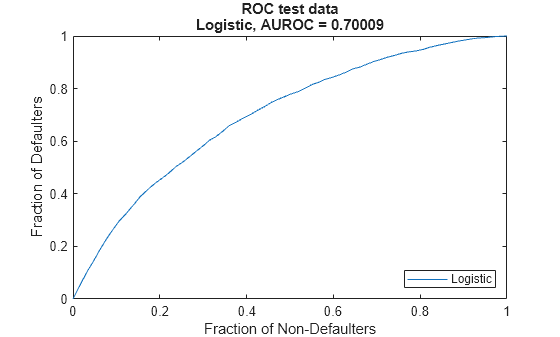
Use modelDiscrimination to measure the ranking of customers by PD.

DiscMeasure = modelDiscrimination(pdModel,data(TestDataInd,:),DataID='test data');
disp(DiscMeasure)

                            AUROC 
                           _______

    Logistic, test data    0.70009

Use modelDiscriminationPlot to visualize the ROC curve.

modelDiscriminationPlot(pdModel,data(TestDataInd,:),DataID='test data');

Use modelCalibration to measure the calibration of the predicted PD values. The modelCalibration function requires a grouping variable and compares the accuracy of the observed default rate in the group with the average predicted PD for the group. For example, you can group by calendar year using the 'Year' variable.

CalMeasure = modelCalibration(pdModel,data(TestDataInd,:),'Year',DataID='test data');
disp(CalMeasure)

                                              RMSE  
                                            ________

    Logistic, grouped by Year, test data    0.000453

Use modelCalibrationPlot to visualize the observed default rates compared to the predicted probabilities of default (PD).

modelCalibrationPlot(pdModel,data(TestDataInd,:),'Year',DataID='test data');

More About

Time Interval for Logistic Models

For Logistic and Probit models, there is a time interval implicit in the data, specifically, in the definition of the default variable. For example, if the default indicator is defined so that it takes the value 1 if there is a default over a 3-month period, the time interval is 3-months. In this case, the predicted PD values are 3-month PD predictions. Then the PD for month 18 would be the conditional probability that there is a default between months 15 and 18, given that there has been no default in the first 15 months.

Because the data input for fitLifetimePDModel is in panel data form, there is an implicit or explicit time stamp for each row, and the time interval used in the default definition should be the same as the time increments between consecutive rows. If there is an optional age variable (AgeVar) in the training data, the time interval should be the same as the age increments (for the same ID) from one row to the next.

Logistic and Probit models infer the time interval from the increments in the age values in the training data when AgeVar is specified and contains numeric values. These models store the time interval value as the TimeInterval property. The predicted PD values returned by predict are consistent with the time interval implicit in the panel training data, which in turn should be the same as the time interval used to define the default variable. The TimeInterval property is also used to validate the data input to the predictLifetime function. For more information, see Validation of Data Input for Lifetime Prediction and Lifetime Prediction and Time Interval.

References

[1] Baesens, Bart, Daniel Roesch, and Harald Scheule. Credit Risk Analytics: Measurement Techniques, Applications, and Examples in SAS. Wiley, 2016.

[2] Bellini, Tiziano. IFRS 9 and CECL Credit Risk Modelling and Validation: A Practical Guide with Examples Worked in R and SAS. San Diego, CA: Elsevier, 2019.

[3] Breeden, Joseph. Living with CECL: The Modeling Dictionary. Santa Fe, NM: Prescient Models LLC, 2018.

[4] Roesch, Daniel and Harald Scheule. Deep Credit Risk: Machine Learning with Python. Independently published, 2020.

Version History

Introduced in R2020b

R2024a: Added TimeInterval name-value argument for Logistic model

The Logistic model supports a TimeInterval name-value argument.

R2023b: Added WeightsVar name-value argument for Logistic model

The Logistic model supports a WeightsVar name-value argument for observation weights.

R2023a: modelAccuracy object function is renamed to modelCalibration function

The modelAccuracy object function is renamed to modelCalibration function. The use of modelAccuracy is discouraged, use modelCalibration instead.

R2023a: modelAccuracyPlot object function is renamed to modelCalibrationPlot function

The modelAccuracyPlot object function is renamed to modelCalibrationPlot function. The use of modelAccuracyPlot is discouraged, use modelCalibrationPlot instead.

R2023a: Model property renamed to UnderlyingModel

The Model property is renamed to UnderlyingModel.