Bandpass Filter Response

This example shows how to compute the time-domain response of a simple bandpass filter. The eight steps involved in computing the time-domain response of a simple bandpass filter are,

1. Use the classic image parameter design to assign inductance and capacitance values to the bandpass filter.

2. Use the circuit, capacitor, and inductor objects with the add function to programmatically construct a Butterworth circuit.

3. Use the setports function to define the circuit as a 2-port network.

4. Use the sparameters function to extract the S-parameters of the 2-port network over a wide frequency range.

5. Use the s2tf function to compute the voltage transfer function from the input to the output.

6. Use the rational object to generate rational fits that capture the ideal RC circuit to a very high degree of accuracy.

7. Use the randn function to create noise in order to create a noisy input voltage waveform.

8. Use the timeresp function to compute the transient response to a noisy input voltage waveform.

Video Walkthrough

For a walkthrough of the example, play the video.

Video Transcript

Loading your interactive content...

Video Player is loading.

Play Video

PlaySkip BackwardSkip Forward

Mute

Current Time 0:00

/

Duration 0:00

Loaded: 0%

0:00

Stream Type LIVE

Seek to live, currently behind liveLIVE

Remaining Time -0:00

 

1x

Playback Rate

• 2x
• 1.5x
• 1.25x
• 1x, selected
• 0.75x
• 0.5x
• 0.25x

Chapters

• Chapters

Descriptions

• descriptions off, selected

Captions

• captions settings, opens captions settings dialog
• captions off, selected

Audio Track

Quality Levels

Picture-in-PictureFullscreen

This is a modal window.

Beginning of dialog window. Escape will cancel and close the window.

Text

ColorWhiteBlackRedGreenBlueYellowMagentaCyanOpacityOpaqueSemi-Transparent

Text Background

ColorBlackWhiteRedGreenBlueYellowMagentaCyanOpacityOpaqueSemi-TransparentTransparent

Caption Area Background

ColorBlackWhiteRedGreenBlueYellowMagentaCyanOpacityTransparentSemi-TransparentOpaque

Font Size

50%75%100%125%150%175%200%300%400%

Text Edge Style

NoneRaisedDepressedUniformDrop shadow

Font Family

Proportional Sans-SerifMonospace Sans-SerifProportional SerifMonospace SerifCasualScriptSmall Caps

ResetDone

Close Modal Dialog

End of dialog window.

Close Modal Dialog

This is a modal window. This modal can be closed by pressing the Escape key or activating the close button.

Design Bandpass Filter Using Image Parameters

The image parameter design is a framework for analytically computing the values of the series and parallel components in the passive filters. For more information on Image Parameters, see "Complete Wireless Design" by Cotter W. Sayre, McGraw-Hill 2008 p. 331.

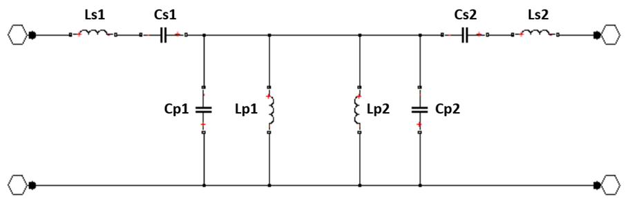
Figure 1: A Butterworth bandpass filter built out of two half-sections.

Generate the component values for a bandpass filter with a lower 3 dB cutoff frequency of 2.4 GHz and an upper 3 dB cutoff frequency of 2.5 GHz.

Ro = 50;
f1C = 2400e6;
f2C = 2500e6;
Ls = (Ro / (pi*(f2C - f1C)))/2;         % Ls1 and Ls2
Cs = 2*(f2C - f1C)/(4*pi*Ro*f2C*f1C);   % Cs1 and Cs2
Lp = 2*Ro*(f2C - f1C)/(4*pi*f2C*f1C);   % Lp1 and Lp2
Cp = (1/(pi*Ro*(f2C - f1C)))/2;         % Cp1 and Cp2

Programmatically Construct Circuit

Before building the circuit using the inductor and capacitor objects, nodes in the circuit are numbered. This is shown in figure 1.

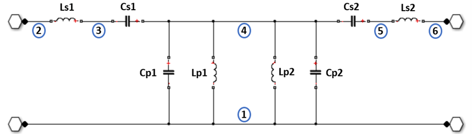
Figure 2: Node numbers added to the Butterworth bandpass filter.

Create a circuit object and populate it with the inductor and the capacitor objects using the add function.

ckt = circuit('butterworthBPF');

add(ckt,[3 2],inductor(Ls));      % Ls1
add(ckt,[4 3],capacitor(Cs));     % Cs1
add(ckt,[5 4],capacitor(Cs));     % Cs2
add(ckt,[6 5],inductor(Ls));      % Ls2

add(ckt,[4 1],capacitor(Cp));     % Cp1
add(ckt,[4 1],inductor(Lp));      % Lp1
add(ckt,[4 1],inductor(Lp));      % Lp2
add(ckt,[4 1],capacitor(Cp));     % Cp2

Extract S-Parameters From 2-Port Network

To extract S-parameters from the circuit object, first use the setports function to define the circuit as a 2-port network.

freq = linspace(2e9,3e9,101);

Use the sparameters function to extract the S-parameters at the frequencies of interest.

setports(ckt,[2 1],[6 1])
S = sparameters(ckt,freq);

Fit Transfer Function of Circuit to Rational Function

Use the s2tf function to generate a transfer function from the S-parameter object.

tfS = s2tf(S);

Use the rational object to fit the transfer function data to a rational function.

fit = rational(freq,tfS);

Verify Rational Fit Approximation

Use the freqresp function to verify that the rational fit approximation has reasonable behavior outside both sides of the fitted frequency range.

widerFreqs = linspace(2e8,5e9,1001);
resp = freqresp(fit,widerFreqs);

Plot to visualize rational fit approximation. The rational fit behaves well outside the fitted frequency range.

figure
semilogy(freq,abs(tfS),widerFreqs,abs(resp),'--','LineWidth',2)
xlabel('Frequency (Hz)');
ylabel('Magnitude');
legend('data','fit');
title('Rational Fit Approximation');

Construct Input Signal to Test Bandpass Filter

To test the bandpass filter, designed by the Image Parameter technique, a sinusoidal signal at 2.45 GHz is recovered from the noisy input signal. The noise input signal is generated by the inclusion of zero-mean random noise and a blocker at 2.35 GHz to the input signal.

Construct an input and a noisy input signal with 8192 samples.

fCenter = 2.45e9;
fBlocker = 2.35e9;
period = 1/fCenter;
sampleTime = period/16;
signalLen = 8192;
t = (0:signalLen-1)'*sampleTime; % 256 periods
input = sin(2*pi*fCenter*t);     % Clean input signal
rng('default')
noise = randn(size(t)) + sin(2*pi*fBlocker*t);
noisyInput = input + noise;      % Noisy input signal

Compute Transient Response to Input Signal

Use the timeresp function to compute the analytic solutions of the state-space.

output = timeresp(fit,noisyInput,sampleTime);

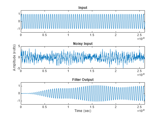
View Input Signal and Filter Response in Time Domain

Plot the input signal, noisy input signal, and the band pass filter output in a figure window.

xmax = t(end)/8;
figure
subplot(3,1,1)
plot(t,input)
axis([0 xmax -1.5 1.5])
title('Input')

subplot(3,1,2)
plot(t,noisyInput)
axis([0 xmax floor(min(noisyInput)) ceil(max(noisyInput))]);
title('Noisy Input');
ylabel('Amplitude (volts)');

subplot(3,1,3)
plot(t,output)
axis([0 xmax -1.5 1.5]);
title('Filter Output');
xlabel('Time (sec)');

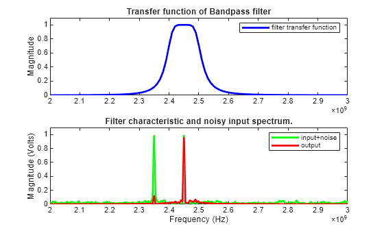
View Input Signal and Filter Response in Frequency Domain

Overlaying the noisy input and the filter response in the frequency domain explains why the filtering operation is successful. Both the blocker signal at 2.35 GHz and much of the noise are significantly attenuated.

NFFT = 2^nextpow2(signalLen); % Next power of 2 from length of y
Y = fft(noisyInput,NFFT)/signalLen;
samplingFreq = 1/sampleTime;
f = samplingFreq/2*linspace(0,1,NFFT/2+1)';
O = fft(output,NFFT)/signalLen;

figure
subplot(2,1,1)
plot(freq,abs(tfS),'b','LineWidth',2)
axis([freq(1) freq(end) 0 1.1]);
legend('filter transfer function');
title('Transfer function of Bandpass filter');
ylabel('Magnitude');

subplot(2,1,2)
plot(f,2*abs(Y(1:NFFT/2+1)),'g',f,2*abs(O(1:NFFT/2+1)),'r','LineWidth',2)
axis([freq(1) freq(end) 0 1.1]);
legend('input+noise','output');
title('Filter characteristic and noisy input spectrum.');
xlabel('Frequency (Hz)');
ylabel('Magnitude (Volts)');

To compute and display this bandpass filter response using RFCKT objects, see Bandpass Filter Response Using RFCKT Objects.