Import and Visualize Ensemble Data in Diagnostic Feature Designer
Diagnostic Feature Designer is an app that allows you to develop features and evaluate potential condition indicators using a multifunction graphical interface.
The app operates on data ensembles. An ensemble is a collection of data sets, created by measuring or simulating a system under varying conditions. An individual data set representing one system under one set of conditions is a member. Diagnostic Feature Designer processes all ensemble members when executing one operation.
This tutorial shows how to import data into Diagnostic Feature Designer and visualize your imported data.
Load Transmission Model Data
This example uses data generated from a transmission system model in Using Simulink to Generate Fault Data. Outputs of the model include:
Vibration measurements from a sensor monitoring casing vibrations
Data from the tachometer, which issues a pulse every time the shaft completes a rotation
Fault codes indicating the presence of a modeled fault
Load the data. The data is a table containing variables logged during multiple simulations of the model under varying conditions. Sixteen members have been extracted from the transmission model logs to form an ensemble. Four of these members represent healthy data, and the remaining 12 members exhibit varying levels of sensor drift.
load dfd_Tutorial dataTable
View this table in your MATLAB® command window.
dataTable =

  16×3 table

        Vibration               Tacho           faultCode
    __________________    __________________    _________

    {6000×1 timetable}    {6000×1 timetable}        0
    {6000×1 timetable}    {6000×1 timetable}        1
    {6000×1 timetable}    {6000×1 timetable}        1
    {6000×1 timetable}    {6000×1 timetable}        1
    {6000×1 timetable}    {6000×1 timetable}        1
    {6000×1 timetable}    {6000×1 timetable}        1
    {6000×1 timetable}    {6000×1 timetable}        1
    {6000×1 timetable}    {6000×1 timetable}        1
    {6000×1 timetable}    {6000×1 timetable}        0
    {6000×1 timetable}    {6000×1 timetable}        0
    {6000×1 timetable}    {6000×1 timetable}        0
    {6000×1 timetable}    {6000×1 timetable}        1
    {6000×1 timetable}    {6000×1 timetable}        1
    {6000×1 timetable}    {6000×1 timetable}        1
    {6000×1 timetable}    {6000×1 timetable}        1
{6000×1 timetable} {6000×1 timetable} 1 Vibration and Tacho are each
represented by a timetable, and all timetables have
the same length. The third variable, faultCode, is the condition
variable. faultCode has a value of 0 for
healthy and 1 for degraded.Open Diagnostic Feature Designer
To open Diagnostic Feature Designer, enter the following command in your command window.
diagnosticFeatureDesigner
Import Data
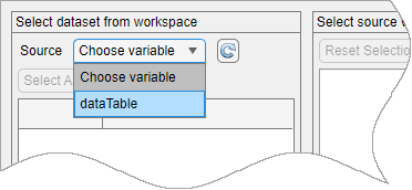
Import the data set that you previously loaded into your MATLAB workspace. To initiate the import process, in the Feature Designer tab, click New Session.

The New Session dialog box opens. From the
Source list in the Select dataset from
workspace pane, select dataTable.
The Select source variables pane of the dialog box now
displays the variables within dataTable. By default, the
app initially selects all source variables for import.
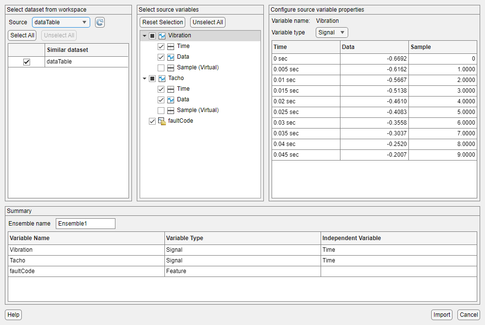
The app extracts the variable names from your member tables and embedded
timetables. The icon next to the Vibration and
Tacho variable names indicates that the app interprets the
variables as time-based signals that each contain Time and
Data variables. You can verify this interpretation in the
Summary pane at the bottom, which displays the variable
name, type, and independent variable for each source-level variable.
A third variable, Sample (Virtual), also appears in the
list, but is not selected and does not appear in Summary. The
import dialog box always includes this variable as an option to allow you to
generate virtual independent variables within the app.
View the properties of Vibration by selecting the
Vibration row.
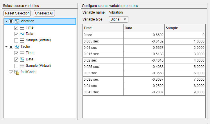
Because the app automatically selects the first variable row for property
configuration, the Configure source variable properties pane
displays the Vibration variable name and the
Signal variable type. For
Vibration, Signal is the only
Variable type option because the vibration data is packaged
in a timetable. Source variable properties also displays a preview of
Vibration data.
Now examine the variable type of faultCode. The icon next to
faultCode, which illustrates a histogram, represents a
feature. Features and condition variables can both be represented by scalars, and
the app cannot distinguish between the two unless the condition variable is a
categorical. To change the variable type, click the faultCode to
open the its properties, and, in Variable type, change
Feature to Condition
Variable.

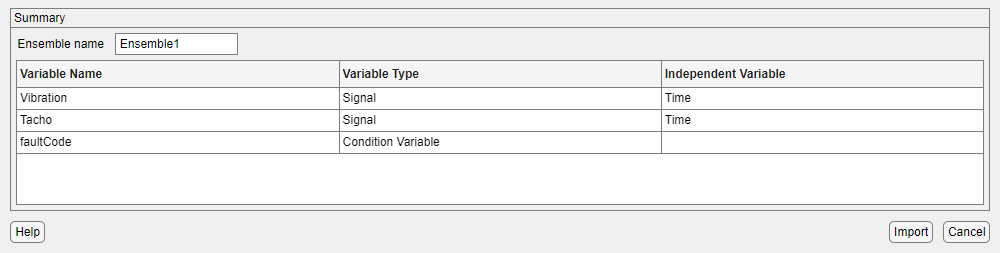
The icon for faultCode now illustrates a paper tag, which
represents a condition variable.
![]()
Confirm the ensemble specification in Summary and click Import.
Your imported variables are now in the Variables pane,
organized into Signal and Condition
Variable types. The color box next to each signal represents that
signal in plots. Since the Vibration and
Tacho signals are both timetables that contain the
signal data in a column named Data, the name
Data appears below both signal names.
Because the Vibration signal is selected, the
Details pane provides additional information about the
signal, including the signal derivation as a direct import and its independent
variable (IV). The Details pane also shows that it is a full
signal rather than a signal that has been processed in frame segments, and that the
signal belongs to a dataset that contains 16 members.

Visualize Data
After you load your signals, plot them and view all your ensemble members
together. To view your vibration signal, in the Vibration signal
in the Variables pane, select Data.
Selecting a signal variable enables the Signal Trace option in
the plot gallery. Click Signal Trace.

The plotting area displays a signal trace plot of all 16 members. As you move the cursor over the data, an indicator in the lower right corner identifies the member your cursor is on. A second indicator provides the fault code value for that member.
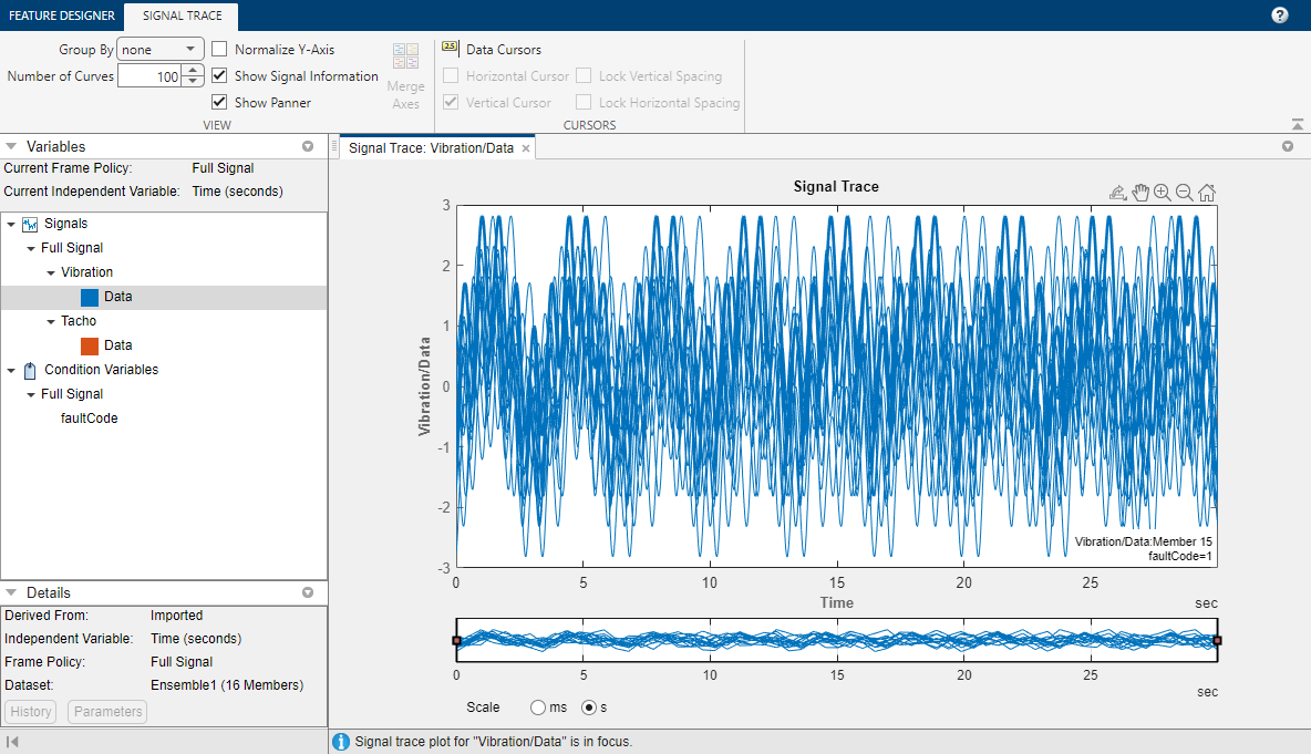
Interact with the trace plot using standard MATLAB plot tools, such as zoom and pan. Access these tools by pointing to the top right edge of the plot. You can also use the specialized options on the Signal Trace tab, which appears when you select the Signal Trace plot.
Explore Your Data Using Signal Trace Options
Explore the data in your plot using options in the Signal Trace tab.

Measure the distance between peaks for the one of the members with high peaks.
Zoom in on the second clusters of peaks. In the panner strip, move the right handle to about 8. Then, move the panner window so that the left handle is at about 4. You now have the second set of peaks within the window.
Pause on the first high peak, and note the member number. The second high peak is a continuation of the same member trace.
Click Data Cursors, and select Vertical Cursor. Place the left cursor over the first high peak and the right cursor over the second peak for that member. The lower right corner of the plot displays the separation
dX.Select Lock Horizontal Spacing. Shift the cursor pair to the right by one peak for the same member. Note that the right cursor is now aligned with the third member peak.
Display Signals with Healthy and Faulty Labels in Different Colors
Show which members have matching faultCode values by using
color coding. In Group By, select
faultCode.

The resulting signal trace shows you that all the highest vibration peaks are associated with data from degraded systems. However, not all the degraded systems have higher peaks.

When you use options like Group By in the plot tab, your
selection is limited to the current plot. To set default plot options for all
your plots, in the Feature Designer tab, click
Plot Options. Then, in Group By,
select faultCode.

All the plots that you create in this tutorial now always group by color. You can override the default settings for a specific plot in the plot tab for that plot.
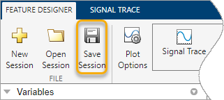
Save your session data. You need this data to run the Process Data and Explore Features in Diagnostic Feature Designer example.
Next Steps
The next step is to explore different ways to characterize your data through features. The example Process Data and Explore Features in Diagnostic Feature Designer guides you through the feature exploration process.
See Also
Topics
- Process Data and Explore Features in Diagnostic Feature Designer
- Rank and Export Features in Diagnostic Feature Designer
- Import Data into Diagnostic Feature Designer
- Explore Ensemble Data and Compare Features Using Diagnostic Feature Designer
- Data Ensembles for Condition Monitoring and Predictive Maintenance
- Condition Indicators for Monitoring, Fault Detection, and Prediction