Measure Intensity Levels Using the Intensity Scope

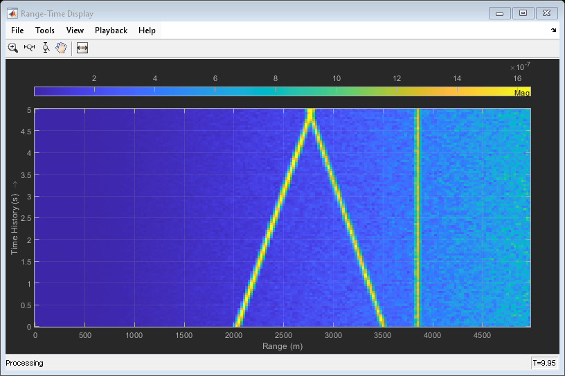
This tutorial shows you how to measure the intensity of signals using the UI of the intensity scope. First, create an intensity scope. You can start with the example below, RTI and DTI Displays in Full Radar Simulation, or you can create your own scope. When this example launches, range-time-intensity (RTI) and Doppler-time-intensity (DTI) display windows open. This tutorial focuses on the RTI display so you can close the DTI window once the processing loop completes. This figure shows the RTI display after processing has completed. The display shows three tracks.

To examine the data, click the Cursor Measurement button in the Toolbar. You see two cursors, each of which is represented by pairs of cross-hairs. To distinguish cursors, one pair consists of solid lines and the second pair consists of dashed lines and are tagged with a 1 or a 2.

Cursor 1 has solid cross-hairs and overlays the intersection of two signal lines. Cursor 2 has dashed cross-hairs and overlays a signal-free region. The Cursor Measurements pane shows the coordinates of the cursors in time and range (labelled X) and the intensities at these positions. Cursor 1 is located at a range of 2775 meters and a time of 3.6 seconds. The signal intensity at this point is 1.989e-6 watts. Cursor 2 is located at a range of 3725 meters and a time of 2.9 seconds. The signal intensity at this point is 3.327e-7 watts. You can move the cursors to any positions of interest and obtain the intensity values.

RTI and DTI Displays in Full Radar Simulation

Open Script

Use the phased.IntensityScope System Object™ to display the detection output of a radar system simulation. The radar scenario contains a stationary single-element monostatic radar and three moving targets.

Set Radar Operating Parameters

Set the maximum range, peak power range resolution, operating frequency, transmitter gain, and target radar cross-section.

max_range = 5000;
range_res = 50;
fc = 10e9;
tx_gain = 20;
peak_power = 5500.0;

Choose the signal propagation speed to be the speed of light, and compute the signal wavelength corresponding to the operating frequency.

c = physconst('LightSpeed');
lambda = c/fc;

Compute the pulse bandwidth from the range resolution. Set the sampling rate, fs, to twice the pulse bandwidth. The noise bandwidth is also set to the pulse bandwidth. The radar integrates a number of pulses set by num_pulse_int. The duration of each pulse is the inverse of the pulse bandwidth.

pulse_bw = c/(2*range_res);
pulse_length = 1/pulse_bw;
fs = 2*pulse_bw;
noise_bw = pulse_bw;
num_pulse_int = 10;

Set the pulse repetition frequency to match the maximum range of the radar.

prf = c/(2*max_range);

Create System Objects for the Model

Choose a rectangular waveform.

waveform = phased.RectangularWaveform('PulseWidth',pulse_length,...
    'PRF',prf,'SampleRate',fs);

Set the receiver amplifier characteristics.

amplifier = phased.ReceiverPreamp('Gain',20,'NoiseFigure',0,...
    'SampleRate',fs,'EnableInputPort',true,'SeedSource','Property',...
    'Seed',2007);
transmitter = phased.Transmitter('Gain',tx_gain,'PeakPower',peak_power,...
    'InUseOutputPort',true);

Specify the radar antenna as a single isotropic antenna.

antenna = phased.IsotropicAntennaElement('FrequencyRange',[5e9 15e9]);

Set up a monostatic radar platform.

radarplatform = phased.Platform('InitialPosition',[0; 0; 0],...
    'Velocity',[0; 0; 0]);

Set up the three target platforms using a single System object.

targetplatforms = phased.Platform(...
    'InitialPosition',[2000.66 3532.63 3845.04; 0 0 0; 0 0 0], ...
    'Velocity',[150 -150 0; 0 0 0; 0 0 0]);

Create the radiator and collector System objects.

radiator = phased.Radiator('Sensor',antenna,'OperatingFrequency',fc);
collector = phased.Collector('Sensor',antenna,'OperatingFrequency',fc);

Set up the three target RCS properties.

targets = phased.RadarTarget('MeanRCS',[1.6 2.2 1.05],'OperatingFrequency',fc);

Create System object to model two-way freespace propagation.

channels= phased.FreeSpace('SampleRate',fs,'TwoWayPropagation',true,...
    'OperatingFrequency',fc);

Define a matched filter.

MFcoef = getMatchedFilter(waveform);
mfilter = phased.MatchedFilter('Coefficients',MFcoef,'GainOutputPort',true);

Create Range and Doppler Bins

Set up the fast-time grid. Fast time is the sampling time of the echoed pulse relative to the pulse transmission time. The range bins are the ranges corresponding to each bin of the fast time grid.

fast_time = unigrid(0,1/fs,1/prf,'[)');
range_bins = c*fast_time/2;

To compensate for range loss, create a time varying gain System Object.

gain = phased.TimeVaryingGain('RangeLoss',2*fspl(range_bins,lambda),...
    'ReferenceLoss',2*fspl(max_range,lambda));

Set up Doppler bins. Doppler bins are determined by the pulse repetition frequency. Create an FFT System object for Doppler processing.

DopplerFFTbins = 32;
DopplerRes = prf/DopplerFFTbins;
fft = dsp.FFT('FFTLengthSource','Property',...
    'FFTLength',DopplerFFTbins);

Create Data Cube

Set up a reduced data cube. Normally, a data cube has fast-time and slow-time dimensions and the number of sensors. Because the data cube has only one sensor, it is two-dimensional.

rx_pulses = zeros(numel(fast_time),num_pulse_int);

Create IntensityScope System Objects

Create two IntensityScope System objects, one for Doppler-time-intensity and the other for range-time-intensity.

dtiscope = phased.IntensityScope('Name','Doppler-Time Display',...
    'XLabel','Velocity (m/sec)', ...
    'XResolution',dop2speed(DopplerRes,c/fc)/2, ...
    'XOffset',dop2speed(-prf/2,c/fc)/2,...
    'TimeResolution',0.05,'TimeSpan',5,'IntensityUnits','Mag');
rtiscope = phased.IntensityScope('Name','Range-Time Display',...
    'XLabel','Range (m)', ...
    'XResolution',c/(2*fs), ...
    'TimeResolution',0.05,'TimeSpan',5,'IntensityUnits','Mag');

Run the Simulation Loop over Multiple Radar Transmissions

Transmit 2000 pulses. Coherently process groups of 10 pulses at a time.

For each pulse:

Update the radar position and velocity radarplatform
Update the target positions and velocities targetplatforms
Create the pulses of a single wave train to be transmitted transmitter
Compute the ranges and angles of the targets with respect to the radar
Radiate the signals to the targets radiator
Propagate the pulses to the target and back channels
Reflect the signals off the target targets
Receive the signal sCollector
Amplify the received signal amplifier
Form data cube

For each set of 10 pulses in the data cube:

Match filter each row (fast-time dimension) of the data cube.
Compute the Doppler shifts for each row (slow-time dimension) of the data cube.

pri = 1/prf;
nsteps = 200;
for k = 1:nsteps
    for m = 1:num_pulse_int
        [ant_pos,ant_vel] = radarplatform(pri);
        [tgt_pos,tgt_vel] = targetplatforms(pri);
        sig = waveform();
        [s,tx_status] = transmitter(sig);
        [~,tgt_ang] = rangeangle(tgt_pos,ant_pos);
        tsig = radiator(s,tgt_ang);
        tsig = channels(tsig,ant_pos,tgt_pos,ant_vel,tgt_vel);
        rsig = targets(tsig);
        rsig = collector(rsig,tgt_ang);
        rx_pulses(:,m) = amplifier(rsig,~(tx_status>0));
    end

    rx_pulses = mfilter(rx_pulses);
    MFdelay = size(MFcoef,1) - 1;
    rx_pulses = buffer(rx_pulses((MFdelay + 1):end), size(rx_pulses,1));
    rx_pulses = gain(rx_pulses);
    range = pulsint(rx_pulses,'noncoherent');
    rtiscope(range);
    dshift = fft(rx_pulses.');
    dshift = fftshift(abs(dshift),1);
    dtiscope(mean(dshift,2));
    radarplatform(.05);
    targetplatforms(.05);
end

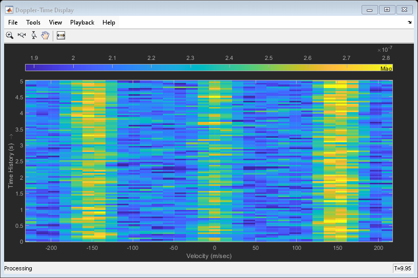
All of the targets lie on the x-axis. Two targets are moving along the x-axis and one is stationary. Because the radar is at the origin, you can read the target speed directly from the Doppler-Time Display window. The values agree with the specified velocities of -150, 150, and 0 m/sec.