evaluateTemperatureGradient
Evaluate temperature gradient of thermal solution at arbitrary spatial locations
Syntax
Description
[
returns the interpolated values of temperature gradients of the thermal model
solution gradTx
,gradTy
]
= evaluateTemperatureGradient(thermalresults
,xq
,yq
)thermalresults
at the 2-D points specified in
xq
and yq
. This syntax is valid for both
the steady-state and transient thermal models.
[___] = evaluateTemperatureGradient(
returns the interpolated values of the temperature gradients at the points specified
in thermalresults
,querypoints
)querypoints
. This syntax is valid for both the steady-state
and transient thermal models.
[___] = evaluateTemperatureGradient(___,
returns the interpolated values of the temperature gradients for the time-dependent
equation at times iT
)iT
. Specify iT
after the
input arguments in any of the previous syntaxes.
The first dimension of gradTx
, gradTy
,
and, in 3-D case, gradTz
corresponds to query points. The
second dimension corresponds to time-steps iT
.
Examples
Temperature Gradients for 2-D Steady-State Thermal Problem
For a 2-D steady-state thermal problem, evaluate temperature gradients at the nodal locations and at the points specified by x
and y
coordinates.
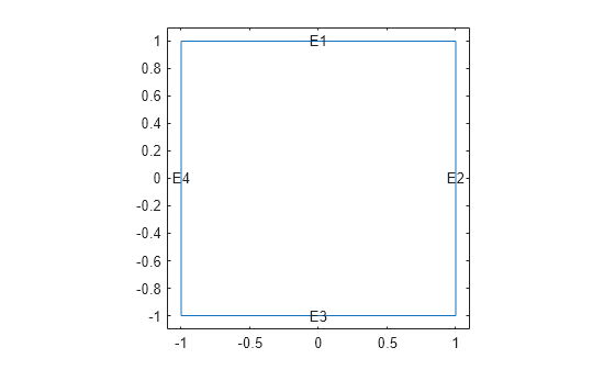
Create and plot a square geometry.
R1 = [3,4,-1,1,1,-1,1,1,-1,-1]'; g = decsg(R1,'R1',('R1')'); pdegplot(g,EdgeLabels="on") xlim([-1.1 1.1]) ylim([-1.1 1.1])
Create an femodel
object for steady-state thermal analysis and include the geometry into the model.
model = femodel(AnalysisType="thermalSteady", ... Geometry=g);
Assuming that this geometry represents an iron plate, the thermal conductivity is .
model.MaterialProperties = ...
materialProperties(ThermalConductivity=79.5);
Apply a constant temperature of 300 K to the bottom of the plate (edge 3).
model.EdgeBC(3) = edgeBC(Temperature=300);
Apply convection on the two sides of the plate (edges 2 and 4).
model.EdgeLoad([2 4]) = ... edgeLoad(ConvectionCoefficient=25,... AmbientTemperature=50);
Mesh the geometry and solve the problem.
model = generateMesh(model); R = solve(model)
R = SteadyStateThermalResults with properties: Temperature: [1529x1 double] XGradients: [1529x1 double] YGradients: [1529x1 double] ZGradients: [] Mesh: [1x1 FEMesh]
The solver finds the temperatures and temperature gradients at the nodal locations. To access these values, use R.Temperature
, R.XGradients
, and so on. For example, plot the temperature gradients at nodal locations.
figure pdeplot(R.Mesh,FlowData=[R.XGradients R.YGradients]);
Create a grid specified by x
and y
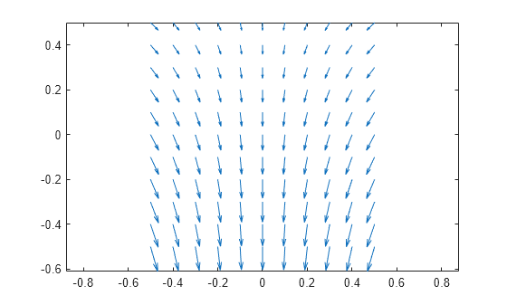
coordinates, and evaluate temperature gradients to the grid.
v = linspace(-0.5,0.5,11);
[X,Y] = meshgrid(v);
[gradTx,gradTy] = ...
evaluateTemperatureGradient(R,X,Y);
Reshape the gradTx
and gradTy
vectors, and plot the resulting temperature gradients.
gradTx = reshape(gradTx,size(X)); gradTy = reshape(gradTy,size(Y)); figure quiver(X,Y,gradTx,gradTy)
Alternatively, you can specify the grid by using a matrix of query points.
querypoints = [X(:) Y(:)]';
[gradTx,gradTy] = ...
evaluateTemperatureGradient(R,querypoints);
gradTx = reshape(gradTx,size(X));
gradTy = reshape(gradTy,size(Y));
figure
quiver(X,Y,gradTx,gradTy)
Temperature Gradients for 3-D Steady-State Thermal Problem
For a 3-D steady-state thermal problem, evaluate temperature gradients at the nodal locations and at the points specified by x
, y
, and z
coordinates.
Create an femodel
object for steady-state thermal analysis and include a block geometry into the model.
model = femodel(AnalysisType="thermalSteady", ... Geometry="Block.stl");
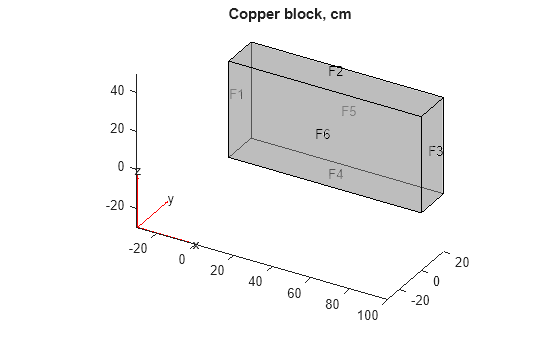
Plot the geometry.
pdegplot(model.Geometry,FaceLabels="on",FaceAlpha=0.5) title("Copper block, cm")
Assuming that this is a copper block, the thermal conductivity of the block is approximately .
model.MaterialProperties = ...
materialProperties(ThermalConductivity=4);
Apply a constant temperature of 373 K to the left side of the block (edge 1) and a constant temperature of 573 K to the right side of the block.
model.FaceBC(1) = faceBC(Temperature=373); model.FaceBC(3) = faceBC(Temperature=573);
Apply a heat flux boundary condition to the bottom of the block.
model.FaceLoad(4) = faceLoad(Heat=-20);
Mesh the geometry and solve the problem.
model = generateMesh(model); R = solve(model)
R = SteadyStateThermalResults with properties: Temperature: [12822x1 double] XGradients: [12822x1 double] YGradients: [12822x1 double] ZGradients: [12822x1 double] Mesh: [1x1 FEMesh]
The solver finds the values of temperatures and temperature gradients at the nodal locations. To access these values, use R.Temperature
, R.XGradients
, and so on.
Create a grid specified by x
, y
, and z
coordinates, and evaluate temperature gradients to the grid.
[X,Y,Z] = meshgrid(1:26:100,1:6:20,1:11:50);
[gradTx,gradTy,gradTz] = ...
evaluateTemperatureGradient(R,X,Y,Z);
Reshape the gradTx
, gradTy
, and gradTz
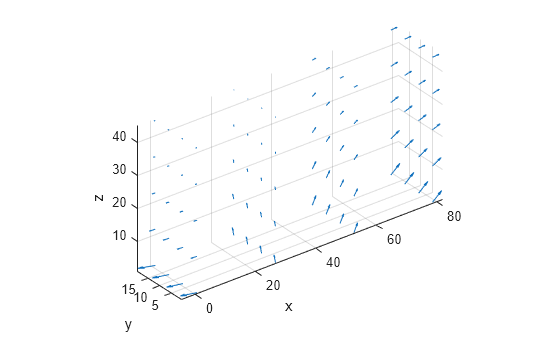
vectors, and plot the resulting temperature gradients.
gradTx = reshape(gradTx,size(X)); gradTy = reshape(gradTy,size(Y)); gradTz = reshape(gradTz,size(Z)); figure quiver3(X,Y,Z,gradTx,gradTy,gradTz) axis equal xlabel("x") ylabel("y") zlabel("z")
Alternatively, you can specify the grid by using a matrix of query points.
querypoints = [X(:) Y(:) Z(:)]'; [gradTx,gradTy,gradTz] = ... evaluateTemperatureGradient(R,querypoints); gradTx = reshape(gradTx,size(X)); gradTy = reshape(gradTy,size(Y)); gradTz = reshape(gradTz,size(Z)); figure quiver3(X,Y,Z,gradTx,gradTy,gradTz) axis equal xlabel("x") ylabel("y") zlabel("z")
Temperature Gradients for Transient Thermal Problem on Square
Solve a 2-D transient heat transfer problem on a square domain and compute temperature gradients at the convective boundary.
Create an femodel
object for transient thermal analysis and include a square geometry into the model.
model = femodel(AnalysisType="thermalTransient", ... Geometry=@squareg);
Plot the geometry.
pdegplot(model.Geometry,EdgeLabels="on")
xlim([-1.1 1.1])
ylim([-1.1 1.1])
Assign the following thermal properties: thermal conductivity is , mass density is , and specific heat is .
model.MaterialProperties = ... materialProperties(ThermalConductivity=100,... MassDensity=7800,... SpecificHeat=500);
Apply the convection boundary condition on the right edge.
model.EdgeLoad(2) = ... edgeLoad(ConvectionCoefficient=5000,... AmbientTemperature=25);
Set the initial conditions: uniform room temperature across domain and higher temperature on the left edge.
model.FaceIC = faceIC(Temperature=25); model.EdgeIC(4) = edgeIC(Temperature=100);
Generate a mesh and solve the problem using 0:1000:200000
as a vector of times.
model = generateMesh(model); tlist = 0:1000:200000; R = solve(model,tlist);
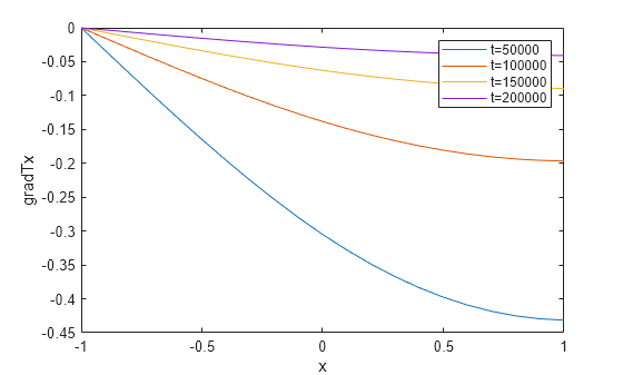
Define a line at convection boundary and compute temperature gradients across that line.
X = -1:0.1:1;
Y = ones(size(X));
[gradTx,gradTy] = ...
evaluateTemperatureGradient(R,X,Y,1:length(tlist));
Plot the interpolated gradient component gradTx
along the x
axis for the following values from the time interval tlist
.
figure t = [51:50:201]; for i = t p(i) = plot(X,gradTx(:,i), ... DisplayName=strcat("t=",num2str(tlist(i)))); hold on end legend(p(t)) xlabel("x") ylabel("gradTx")
Input Arguments
thermalresults
— Solution of thermal problem
SteadyStateThermalResults
object | TransientThermalResults
object
Solution of a thermal problem, specified as a SteadyStateThermalResults
object or
a TransientThermalResults
object.
Create thermalresults
using the
solve
function.
xq
— x-coordinate query points
real array
x-coordinate query points, specified as a real array.
evaluateTemperatureGradient
evaluates temperature
gradient at the 2-D coordinate points [xq(i) yq(i)]
or at
the 3-D coordinate points [xq(i) yq(i) zq(i)]
. So
xq
, yq
, and (if present)
zq
must have the same number of entries.
evaluateTemperatureGradient
converts query points to
column vectors xq(:)
, yq(:)
, and (if
present) zq(:)
. It returns the temperature gradient in a
form of a column vector of the same size. To ensure that the dimensions of
the returned solution is consistent with the dimensions of the original
query points, use reshape
. For example, use
gradTx = reshape(gradTx,size(xq))
.
Data Types: double
yq
— y-coordinate query points
real array
y-coordinate query points, specified as a real array.
evaluateTemperatureGradient
evaluates the
temperature gradient at the 2-D coordinate points [xq(i)
yq(i)]
or at the 3-D coordinate points [xq(i) yq(i)
zq(i)]
. So xq
, yq
, and
(if present) zq
must have the same number of
entries.
evaluateTemperatureGradient
converts query points to
column vectors xq(:)
, yq(:)
, and (if
present) zq(:)
. It returns the temperature gradient in a
form of a column vector of the same size. To ensure that the dimensions of
the returned solution is consistent with the dimensions of the original
query points, use reshape
. For example, use
gradTy = reshape(gradTy,size(yq))
.
Data Types: double
zq
— z-coordinate query points
real array
z-coordinate query points, specified as a real array.
evaluateTemperatureGradient
evaluates the
temperature gradient at the 3-D coordinate points [xq(i) yq(i)
zq(i)]
. So xq
, yq
,
and zq
must have the same number of entries.
evaluateTemperatureGradient
converts query points to
column vectors xq(:)
, yq(:)
, and (if
present) zq(:)
. It returns the temperature gradient in a
form of a column vector of the same size. To ensure that the dimensions of
the returned solution is consistent with the dimensions of the original
query points, use reshape
. For example, use
gradTz = reshape(gradTz,size(zq))
.
Data Types: double
querypoints
— Query points
real matrix
Query points, specified as a real matrix with either two rows for 2-D
geometry, or three rows for 3-D geometry. evaluateTemperatureGradient
evaluates the temperature
gradient at the coordinate points querypoints(:,i)
, so
each column of querypoints
contains exactly one 2-D or
3-D query point.
Example: For 2-D geometry, querypoints = [0.5 0.5 0.75 0.75; 1 2 0
0.5]
Data Types: double
iT
— Time indices
vector of positive integers
Time indices, specified as a vector of positive integers. Each
entry in iT
specifies a time index.
Example: iT = 1:5:21
specifies every fifth
time-step up to 21.
Data Types: double
Output Arguments
gradTx
— x-component of the temperature gradient
matrix
x-component of the temperature gradient, returned as a
matrix. For query points that are outside the geometry,
gradTx
= NaN
.
gradTy
— y-component of the temperature gradient
matrix
y-component of the temperature gradient, returned as a
matrix. For query points that are outside the geometry,
gradTy
= NaN
.
gradTz
— z-component of the temperature gradient
matrix
z-component of the temperature gradient, returned as a
matrix. For query points that are outside the geometry,
gradTz
= NaN
.
Version History
Introduced in R2017a
See Also
Objects
Functions
MATLAB Command
You clicked a link that corresponds to this MATLAB command:
Run the command by entering it in the MATLAB Command Window. Web browsers do not support MATLAB commands.
Select a Web Site
Choose a web site to get translated content where available and see local events and offers. Based on your location, we recommend that you select: .
You can also select a web site from the following list:
How to Get Best Site Performance
Select the China site (in Chinese or English) for best site performance. Other MathWorks country sites are not optimized for visits from your location.
Americas
- América Latina (Español)
- Canada (English)
- United States (English)
Europe
- Belgium (English)
- Denmark (English)
- Deutschland (Deutsch)
- España (Español)
- Finland (English)
- France (Français)
- Ireland (English)
- Italia (Italiano)
- Luxembourg (English)
- Netherlands (English)
- Norway (English)
- Österreich (Deutsch)
- Portugal (English)
- Sweden (English)
- Switzerland
- United Kingdom (English)