Write Portable GPU Code

This example shows how to write robust code that can run on machines with or without a GPU.

Writing code that can run on either a CPU or a GPU allows you to run it on different machines and share it with collaborators, while ensuring that anyone with a GPU who runs the code can benefit from GPU acceleration.

Define Function That Runs on CPU

Define a function, matrixOperationsCPU, that performs these steps:

Computes the inverse of an input matrix A
Computes the matrix square root of the inverse
Creates a matrix of ones, the same size as input matrix A
Multiplies the matrix square root of the inverse by the matrix of ones

function D = matrixOperationsCPU(A)

% Compute inverse.
B = inv(A);

% Compute matrix square root.
C = sqrtm(B);

% Create matrix of ones with the same size as A.
sz = size(A);
R = ones(sz);

% Multiply matrix square root by matrix of ones.
D = R*C;

end

Check that the function works as expected on the CPU. The function runs on the CPU by default.

A = [1 0 2; -1 5 0; 0 3 -9];
C = matrixOperationsCPU(A)

C = 3×3 complex

    1.1161 - 0.0055i    0.4269 - 0.0555i    0.2283 + 0.2597i
    1.1161 - 0.0055i    0.4269 - 0.0555i    0.2283 + 0.2597i
    1.1161 - 0.0055i    0.4269 - 0.0555i    0.2283 + 0.2597i

Edit Function to Run on GPU or CPU

There are several options for editing the function to be able to run on either a CPU or GPU. The most common pattern is to allow the type of the input data to dictate if the GPU is used or not. In other words, if the input data is a gpuArray then run the function on a GPU, and otherwise run the function on a CPU.

There are several functions and syntaxes that are useful for creating functions that can run on a GPU or CPU. With the exception of gpuArray, none of these features require Parallel Computing Toolbox™.

gpuArray and gather — Use the gpuArray function to move data to GPU memory. Use gather to retrieve data from GPU memory.
like syntaxes — The like=p syntaxes of many data creation functions, such as rand and zeros, make the function return data of the same type and complexity of an existing array p.
canUseGPU — The canUseGPU function verifies that a supported GPU is available and that Parallel Computing Toolbox is installed and licensed for use.
isa — The isa function determines whether the input data has a specified data type, such as gpuArray, double, or single.

The matrixOperationsCPU function throws an error if input matrix A is a gpuArray, because the sqrtm function does not support gpuArray input. If a function supports gpuArray input, this is indicated in the Extended Capabilities section of the function reference page.

Define a new function, matrixOperations, that performs the same operations as matrixOperationsCPU and contains additional code for handling gpuArray input. The function:

Gathers the matrix B from the GPU before using the sqrtm function. If B is not a gpuArray, then the gather function has no effect.
Creates a matrix of ones R with the same type as the input matrix A. If A is a gpuArray, the function creates the matrix R directly on the GPU.

function D = matrixOperations(A)

% Compute inverse.
B = inv(A);

% Compute matrix square root.
B = gather(B);
C = sqrtm(B);

% Create a matrix of ones with the same type and size as A.
sz = size(A);
R = ones(sz,like=A);

% Multiply matrix square root by matrix of ones.
D = R*C;

end

Check that the output of the function is the same regardless of whether you run it on the CPU or on the GPU.

C = matrixOperations(A)

C = 3×3 complex

    1.1161 - 0.0055i    0.4269 - 0.0555i    0.2283 + 0.2597i
    1.1161 - 0.0055i    0.4269 - 0.0555i    0.2283 + 0.2597i
    1.1161 - 0.0055i    0.4269 - 0.0555i    0.2283 + 0.2597i

A = gpuArray(A);
CGPU = matrixOperations(A)

CGPU =

   1.1161 - 0.0055i   0.4269 - 0.0555i   0.2283 + 0.2597i
   1.1161 - 0.0055i   0.4269 - 0.0555i   0.2283 + 0.2597i
   1.1161 - 0.0055i   0.4269 - 0.0555i   0.2283 + 0.2597i

Check that the output of the function is a gpuArray when the input is a gpuArray.

isa(CGPU,"gpuArray")

ans = logical
   1

Use `gpuArray` Function in Portable Code

To use gpuArray inside portable code, only call it inside a conditional statement that is only run if you have a supported GPU and Parallel Computing Toolbox. For example, create a matrix and convert it to a gpuArray only if canUseGPU returns 1 (true).

X = [2 7 9; 2 3 4; 7 1 3];

if canUseGPU
    X = gpuArray(X);
end

Define Function to Solve Two-Dimensional Wave Equation (Optional)

In this section, you see a more complete and complicated example of code that is able to run on a CPU or a GPU.

The waveEquation function solves the two-dimensional wave equation using spectral methods [1]. The function is defined at the end of this example and it uses the cast and zeros functions with the like syntax to ensure that data is a gpuArray if the input data is a gpuArray. This allows the waveEquation function to run on a CPU or a GPU depending on the type of the input data.

The two-dimensional wave equation can be written as

$\frac{\partial^{2}}{\partial t^{2}} u = \frac{\partial^{2}}{\partial x^{2}} u + \frac{\partial^{2}}{\partial y^{2}} u$ ,

where $u = u (x, y, t)$ is a scalar field, $x$ and $y$ are spatial coordinates, and $t$ is the time coordinate. The function assumes that $u = 0$ on the boundaries of a 2-D grid.

Specify the grid size and create a mesh grid using Chebyshev points.

gridSize = 64;

x = cos(pi*(0:gridSize)/gridSize);
y = x';

[xx,yy] = meshgrid(x,y);

Define conditions for two time steps.

vv = exp(-40*((xx-.4).^2 + yy.^2));
vv0 = vv;

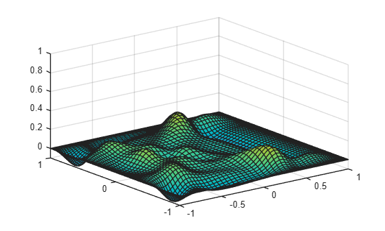
Solve the equation over 1000 time steps on the CPU. The type of the input vv determines whether the function performs the calculations on the CPU or the GPU. Specifically, if vv is a gpuArray, then the function performs the calculations on the GPU.

numSteps = 2000;
[vv,xx,yy] = waveEquation(vv,vv0,GridSize=gridSize,NumSteps=numSteps,Plots=true);

Compare how long it takes to run the function on a CPU versus on a GPU. Use the timeit function to time CPU execution and the gputimeit function to time GPU execution. gputimeit is preferable to timeit for functions that use the GPU, because it checks that all operations on the GPU have finished before recording the time and compensates for overheads. timeit offers greater precision for operations that do not use a GPU. Run the function on a 256-by-256 grid for 1000 time steps.

gridSize = 256;
numSteps = 1000;
x = cos(pi*(0:gridSize)/gridSize);
y = x';

[xx,yy] = meshgrid(x,y);

vv = exp(-40*((xx-.4).^2 + yy.^2));
vv0 = vv;
tCPU = timeit(@() waveEquation(vv,vv0,GridSize=gridSize,NumSteps=numSteps,Plots=false),3)

tCPU = 
18.7529

vv = gpuArray(vv);
tGPU = gputimeit(@() waveEquation(vv,vv0,GridSize=gridSize,NumSteps=numSteps,Plots=false),3)

tGPU = 
0.8554

disp("Speedup when using GPU: " + round(tCPU/tGPU,1) + "x")

Speedup when using GPU: 21.9x

When you run this code, the performance improvement will strongly depend on your hardware.

Supporting Functions

`waveEquation` Function

The waveEquation function solves the two-dimensional wave equation using spectral methods [1]. The function takes the state of the system at two previous time steps, and optionally the grid size, number of steps to solve for, and plotting options as input.

The waveEquation function uses the cast and zeros functions with the like syntax, specifying the input data as a prototype array. This allows the waveEquation function to run on a CPU or a GPU, in single precision or double precision, depending on the type of the input data.

function [vv,xx,yy] = waveEquation(vv,vv0,NameValueArgs)

arguments
    % Initial conditions.
    vv  (:,:) {mustBeFloat}
    vv0 (:,:) {mustBeFloat}

    % Name-value arguments.
    NameValueArgs.GridSize (1,1) double {mustBePositive,mustBeInteger} = 64
    NameValueArgs.NumSteps (1,1) double {mustBeNonnegative,mustBeInteger} = 1000
    NameValueArgs.Plots (1,1) logical = true
    NameValueArgs.PlottingFrequency (1,1) double {mustBePositive,mustBeInteger} = 20;
end

% Make GridSize the same type as vv. If vv is a gpuArray, then MATLAB performs subsequent
% operations involving GridSize, including the colon operator, on the GPU.
NameValueArgs.GridSize = cast(NameValueArgs.GridSize,like=vv);

% Set up grid using Chebyshev points.
x = cos(pi*(0:NameValueArgs.GridSize)/NameValueArgs.GridSize);
y = x';
[xx,yy] = meshgrid(x,y);

% Calculate time step.
dt = 6/NameValueArgs.GridSize^2;

% Initialize weights used for spectral differentiation via FFT.
ii = 2:NameValueArgs.GridSize;
index1 = 1i*[0:NameValueArgs.GridSize-1 0 1-NameValueArgs.GridSize:-1];
index2 = -[0:NameValueArgs.GridSize 1-NameValueArgs.GridSize:-1].^2;

W1T = repmat(index1,NameValueArgs.GridSize-1,1);
W2T = repmat(index2,NameValueArgs.GridSize-1,1);
W3T = repmat(index1.',1,NameValueArgs.GridSize-1);
W4T = repmat(index2.',1,NameValueArgs.GridSize-1);

WuxxT1 = repmat((1./(1-x(ii).^2)),NameValueArgs.GridSize-1,1);
WuxxT2 = repmat(x(ii)./(1-x(ii).^2).^(3/2),NameValueArgs.GridSize-1,1);
WuyyT1 = repmat(1./(1-y(ii).^2),1,NameValueArgs.GridSize-1);
WuyyT2 = repmat(y(ii)./(1-y(ii).^2).^(3/2),1,NameValueArgs.GridSize-1);

uxx=zeros(NameValueArgs.GridSize+1,NameValueArgs.GridSize+1,like=vv);
uyy=zeros(NameValueArgs.GridSize+1,NameValueArgs.GridSize+1,like=vv);

for step = 1:NameValueArgs.NumSteps
    V = [vv(ii,:) vv(ii,NameValueArgs.GridSize:-1:2)];
    U = real(fft(V.')).';

    W1test = (U.*W1T).';
    W2test = (U.*W2T).';
    W1 = (real(ifft(W1test))).';
    W2 = (real(ifft(W2test))).';

    % Calculate second derivative in x.
    uxx(ii,ii) = W2(:,ii).* WuxxT1 - W1(:,ii).*WuxxT2;
    uxx([1,NameValueArgs.GridSize+1],[1,NameValueArgs.GridSize+1]) = 0;

    V = [vv(:,ii); vv((NameValueArgs.GridSize:-1:2),ii)];
    U = real(fft(V));

    W1 = real(ifft(U.*W3T));
    W2 = real(ifft(U.*W4T));

    % Calculating second derivative in y
    uyy(ii,ii) = W2(ii,:).* WuyyT1 - W1(ii,:).*WuyyT2;
    uyy([1,NameValueArgs.GridSize+1],[1,NameValueArgs.GridSize+1]) = 0;

    % Compute new values using 2nd order central finite difference in time.
    vvnew = 2*vv - vv0 + dt*dt*(uxx+uyy);
    vv0 = vv;
    vv = vvnew;

    % Plot result.
    if NameValueArgs.Plots==true && (step==1 || step==NameValueArgs.NumSteps || mod(step,NameValueArgs.PlottingFrequency)==0)
        updatePlot(xx,yy,vv,step)
    end

end

end

`updatePlot` Function

The waveEquation function calls the updatePlot function to generate and update a surface plot of the scalar field. The updatePlot function takes the grid coordinates xx and yy, the calculated solution vv, and the current step number step. After the first step, the function initializes a surface plot and sets appropriate axis and color limits. For subsequent steps, the function updates the plot with the current values.

function updatePlot(xx,yy,vv,step)

if step == 1
    % Initialize plot.
    figure
    ax = axes;
    surf(ax,xx,yy,vv);
    axis([-1 1 -1 1 -0.1 1]);
    clim([-0.5 0.5]);
    ax.Clipping = "off";
else
    % Update plot.
    ax = gca;
    surface = ax.Children;
    surface.ZData = gather(vv);
end

drawnow
end

References

[1] Trefethen, Lloyd N. Spectral Methods in MATLAB. Software, Environments, Tools. Society for Industrial and Applied Mathematics, 2000.

Write Portable GPU Code

Define Function That Runs on CPU

Edit Function to Run on GPU or CPU

Use `gpuArray` Function in Portable Code

Define Function to Solve Two-Dimensional Wave Equation (Optional)

Supporting Functions

`waveEquation` Function

`updatePlot` Function

References

See Also

Topics

Write Portable GPU Code

Define Function That Runs on CPU

Edit Function to Run on GPU or CPU

Use gpuArray Function in Portable Code

Define Function to Solve Two-Dimensional Wave Equation (Optional)

Supporting Functions

waveEquation Function

updatePlot Function

References

See Also

Topics

Use `gpuArray` Function in Portable Code

`waveEquation` Function

`updatePlot` Function