Visualizing Vector Volume Data

Lines, Particles, Ribbons, Streams, Tubes, and Cones

Vector volume data contains more information than scalar data because each coordinate point in the data set has three values associated with it. These values define a vector that represents both a magnitude and a direction. The velocity of fluid flow is an example of vector data.

A number of techniques are useful for visualizing vector data:

Stream lines trace the path that a massless particle immersed in the vector field would follow.
Stream particles are markers that trace stream lines and are useful for creating stream line animations.
Stream ribbons are similar to stream lines, except that the width of the ribbons enables them to indicate twist. Stream ribbons are useful to indicate curl angular velocity.
Stream tubes are similar to stream lines, but you can also control the width of the tube. Stream tubes are useful for displaying the divergence of a vector field.
Cone plots represent the magnitude and direction of the data at each point by displaying a conical arrowhead or an arrow.

It is typically the case that these functions best elucidate the data when used in conjunction with other visualization techniques, such as contours, slice planes, and isosurfaces. The examples in this section illustrate some of these techniques.

Using Scalar Techniques with Vector Data

Visualization techniques such as contour slices, slice planes, and isosurfaces require scalar volume data. You can use these techniques with vector data by taking the magnitude of the vectors. For example, the wind data set returns three coordinate arrays and three vector component arrays, u, v, w. In this case, the magnitude of the velocity vectors equals the wind speed at each corresponding coordinate point in the volume.

wind_speed = sqrt(u.^2 + v.^2 + w.^2);

The array wind_speed contains scalar values for the volume data. The usefulness of the information produced by this approach, however, depends on what physical phenomenon is represented by the magnitude of your vector data.

Specifying Starting Points for Stream Plots

Stream plots (stream lines, ribbons, tubes, and cones or arrows) illustrate the flow of a 3-D vector field. The MATLAB^® stream-plotting functions (streamline, streamribbon, streamtube, coneplot, stream2, stream3) all require you to specify the point at which you want to begin each stream trace.

Determining the Starting Points

Generally, knowledge of your data's characteristics helps you select the starting points. Information such as the primary direction of flow and the range of the data coordinates helps you decide where to evaluate the data.

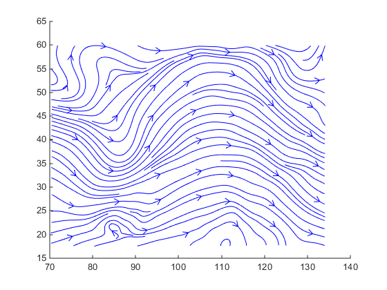
The streamslice function is useful for exploring your data. For example, these statements draw a slice through the vector field at a z value midway in the range.

load wind
zmax = max(z(:)); zmin = min(z(:));
streamslice(x,y,z,u,v,w,[],[],(zmax-zmin)/2)

This stream slice plot indicates that the flow is in the positive x-direction and also enables you to select starting points in both x and y. You could create similar plots that slice the volume in the x-z plane or the y-z plane to gain further insight into your data's range and orientation.

Specifying Arrays of Starting-Point Coordinates

To specify the starting point for one stream line, you need the x-, y-, and z-coordinates of the point. The meshgrid command provides a convenient way to create arrays of starting points. For example, you could select the following starting points from the wind data displayed in the previous stream slice.

[sx,sy,sz] = meshgrid(80,20:10:50,0:5:15);

This statement defines the starting points as all lying on x = 80, y ranging from 20 to 50, and z ranging from 0 to 15. You can use plot3 to display the locations.

plot3(sx(:),sy(:),sz(:),'*r');
axis(volumebounds(x,y,z,u,v,w))
grid on 
set(gca,'BoxStyle','full','Box','on')
daspect([2 2 1])

You do not need to use 3-D arrays, such as those returned by meshgrid, but the size of each array must be the same, and meshgrid provides a convenient way to generate arrays when you do not have an equal number of unique values in each coordinate. You can also define starting-point arrays as column vectors. For example, meshgrid returns 3-D arrays:

[sx,sy,sz] = meshgrid(80,20:10:50,0:5:15);
whos

  Name      Size             Bytes  Class     Attributes

  sx        4x1x4              128  double              
  sy        4x1x4              128  double              
  sz        4x1x4              128  double

In addition, you could use 16-by-1 column vectors with the corresponding elements of the three arrays composing the coordinates of each starting point. (This is the equivalent of indexing the values returned by meshgrid as sx(:), sy(:), and sz(:).)

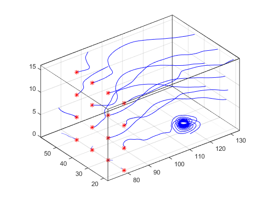
For example, adding the stream lines to the starting points produces:

streamline(x,y,z,u,v,w,sx(:),sy(:),sz(:))

Accessing Subregions of Volume Data

The subvolume function provides a simple way to access subregions of a volume data set. subvolume enables you to select regions of interest based on limits rather than using the colon operator to index into the 3-D arrays that define volumes. Consider the following two approaches to creating the data for a subvolume — indexing with the colon operator and using subvolume.

Indexing with the Colon Operator

When you index the arrays, you work with values that specify the elements in each dimension of the array.

load wind
xsub = x(1:10,20:30,1:7);
ysub = y(1:10,20:30,1:7);
zsub = z(1:10,20:30,1:7);
usub = u(1:10,20:30,1:7);
vsub = v(1:10,20:30,1:7);
wsub = w(1:10,20:30,1:7);

Using the subvolume Function

subvolume enables you to use coordinate values that you can read from the axes. For example:

lims = [100.64 116.67 17.25 28.75 -0.02 6.86];
[xsub,ysub,zsub,usub,vsub,wsub] = subvolume(x,y,z,u,v,w,lims);

You can then use the subvolume data as inputs to any function requiring vector volume data.