stream2
Compute 2-D streamline data
Description
computes 2-D streamline data using the specified options, defined as a one- or two-element
vector with the form XY
= stream2(___,options
)step
or [step maxvert]
, where
step
is the step size in data units for interpolating the vector data
and maxvert
is the maximum number of vertices in a streamline. Use this
argument with any of the input argument combinations from the previous syntaxes.
Examples
Compute 2-D Streamlines
Load the wind
data set, which contains measurements of air current over regions of North America.
3-D arrays
x
andy
represent the locations of air current measurements.3-D arrays
u
andv
represent the velocity of the air current in 3-D vector fields.
Use the fifth page of the arrays. Define the starting position of four hypothetical particles. In this case, the four starting locations are (80, 20), (80, 30), (80, 40), and (80, 50).
load wind
x5 = x(:,:,5);
y5 = y(:,:,5);
u5 = u(:,:,5);
v5 = v(:,:,5);
[startX,startY] = meshgrid(80,20:10:50);
Compute the 2-D streamline vertex data for a hypothetical particle placed into the air current with stream2
.
verts = stream2(x5,y5,u5,v5,startX,startY);
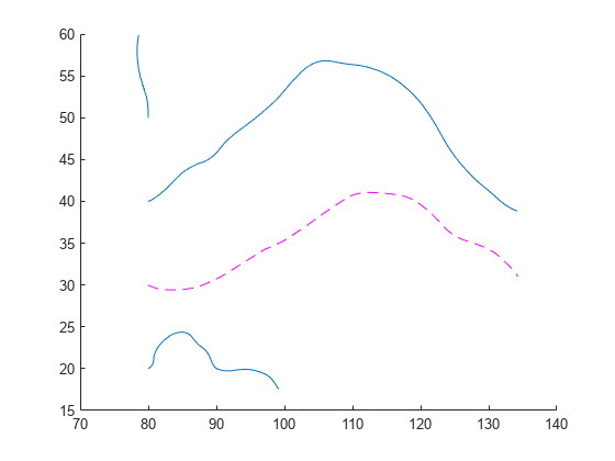
Visualize the 2-D matrix of vector fields by calling streamline
. Return the line objects in the variable lineobj
, so you can change their properties later.
lineobj = streamline(verts);
To change aspects of a particular line, set properties on one of the returned line objects. For example, change the color of the second line to magenta and change its style to dashed.
lineobj(2).Color = "m"; lineobj(2).LineStyle = "--";
Specify Step Size for 2-D Streamlines
Load the wind
data set, which contains measurements of air current over regions of North America.
3-D arrays
x
andy
represent the locations of air current measurements.3-D arrays
u
andv
represent the velocity of the air current in 3-D vector fields..
Use the fifth page of the arrays. Define the starting position of four hypothetical particles. In this case, the four starting locations are (80, 20), (80, 30), (80, 40), and (80, 50).
load wind
x5 = x(:,:,5);
y5 = y(:,:,5);
u5 = u(:,:,5);
v5 = v(:,:,5);
[startX,startY] = meshgrid(80,20:10:50);
Decrease the streamline resolution by increasing the step size from the default of 0.1 to 3.
step = 3;
Compute the 2-D streamline vertex data for a hypothetical particle placed into the air current with stream2
and step
.
verts = stream2(x5,y5,u5,v5,startX,startY,step);
Visualize the 2-D matrix of vector fields with streamline
. The larger step size results in a lower resolution streamline.
streamline(verts)
Specify Maximum Number of Vertices for 2-D Streamlines
Load the wind
data set, which contains measurements of air current over regions of North America.
3-D arrays
x
andy
represent the locations of air current measurements.3-D arrays
u
andv
represent the velocity of the air current in 3-D vector fields.
Use the fifth page of the arrays. Define the starting position of four hypothetical particles. In this case, the four starting locations are (80, 20), (80, 30), (80, 40), and (80, 50).
load wind
x5 = x(:,:,5);
y5 = y(:,:,5);
u5 = u(:,:,5);
v5 = v(:,:,5);
[startX,startY] = meshgrid(80,20:10:50);
Increase the streamline resolution by decreasing the step size from the default of 0.1 to 0.01.
step = 0.01;
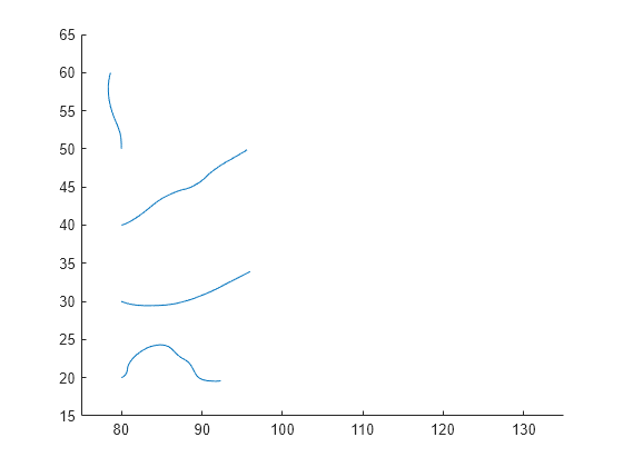
Set the maximum number of vertices so that computation ends after the first 1,000 vertices are calculated.
maxvert = 1000;
Compute the 2-D streamline vertex data for a hypothetical particle placed into the air current with stream2
, step
, and maxvert
.
verts = stream2(x5,y5,u5,v5,startX,startY,[step maxvert]);
Visualize the 2-D matrix of vector fields with streamline
. Show the full range of data values by setting the axis limits. The streamlines end after 1,000 vertices are calculated, so the streamlines stop before showing the full range of data.
streamline(verts) xlim([75 135]) ylim([15 65])
Input Arguments
X
— x-axis coordinates of vector data
2-D array
x-axis coordinates of vector data, specified as a 2-D array. It
must be monotonic, but does not need to be uniformly spaced. X
must
be the same size as Y
, U
, and
V
.
You can use the meshgrid
function to create
X
.
Y
— y-axis coordinates of vector data
2-D array
y-axis coordinates of vector data, specified as a 2-D array. It
must be monotonic, but does not need to be uniformly spaced. Y
must
be the same size as X
, U
, and
V
.
You can use the meshgrid
function to create
Y
.
U
— x-components of vector data
2-D array
x-components of vector data, specified as a 2-D array.
U
must be the same size as X
,
Y
, and V
.
V
— y-components of vector data
2-D array
y-components of vector data, specified as a 2-D array.
V
must be the same size as X
,
Y
, and U
.
startX
— x-axis streamline starting positions
scalar | vector | matrix
x-axis streamline starting positions, specified as a vector or
matrix. startX
must be a scalar or be the same size as
startY
.
startY
— y-axis streamline starting positions
scalar | vector | matrix
y-axis streamline starting positions, specified as a vector or
matrix. startY
must be a scalar or be the same size as
startX
.
options
— Streamline options
[0.1 10000] (default) | one-element vector | two-element vector
Streamline options, specified as a one- or two-element vector with one of the following forms:
step
[step maxvert]
step
is the step size used to adjust the streamline resolution
and determine the vertex locations for which streamline velocity is interpolated.
maxvert
is the maximum number of vertices calculated for a
streamline before computation is complete.
The default step-size is 0.1
, and the default maximum number of
vertices in a streamline is 10,000
.
Extended Capabilities
GPU Arrays
Accelerate code by running on a graphics processing unit (GPU) using Parallel Computing Toolbox™.
The stream2
function
supports GPU array input with these usage notes and limitations:
This function accepts GPU arrays, but does not run on a GPU.
For more information, see Run MATLAB Functions on a GPU (Parallel Computing Toolbox).
Distributed Arrays
Partition large arrays across the combined memory of your cluster using Parallel Computing Toolbox™.
Usage notes and limitations:
This function operates on distributed arrays, but executes in the client MATLAB®.
For more information, see Run MATLAB Functions with Distributed Arrays (Parallel Computing Toolbox).
Version History
Introduced before R2006a
MATLAB Command
You clicked a link that corresponds to this MATLAB command:
Run the command by entering it in the MATLAB Command Window. Web browsers do not support MATLAB commands.
Select a Web Site
Choose a web site to get translated content where available and see local events and offers. Based on your location, we recommend that you select: .
You can also select a web site from the following list:
How to Get Best Site Performance
Select the China site (in Chinese or English) for best site performance. Other MathWorks country sites are not optimized for visits from your location.
Americas
- América Latina (Español)
- Canada (English)
- United States (English)
Europe
- Belgium (English)
- Denmark (English)
- Deutschland (Deutsch)
- España (Español)
- Finland (English)
- France (Français)
- Ireland (English)
- Italia (Italiano)
- Luxembourg (English)
- Netherlands (English)
- Norway (English)
- Österreich (Deutsch)
- Portugal (English)
- Sweden (English)
- Switzerland
- United Kingdom (English)