Main Content

divergence

Compute divergence of vector field

Description

div = divergence(X,Y,Z,Fx,Fy,Fz) computes the numerical divergence of a 3-D vector field with vector components Fx, Fy, and Fz.

The arrays X, Y, and Z, which define the coordinates for the vector components Fx, Fy, and Fz, must be monotonic, but do not need to be uniformly spaced. X, Y, and Z must be 3-D arrays of the same size, which can be produced by meshgrid.

example

div = divergence(Fx,Fy,Fz) assumes a default grid of sample points. The default grid points X, Y, and Z are determined by the expression [X,Y,Z] = meshgrid(1:n,1:m,1:p), where [m,n,p] = size(Fx). Use this syntax when you want to conserve memory and are not concerned about the absolute distances between points.

div = divergence(X,Y,Fx,Fy) computes the numerical divergence of a 2-D vector field with vector components Fx and Fy.

The matrices X and Y, which define the coordinates for Fx and Fy, must be monotonic, but do not need to be uniformly spaced. X and Y must be 2-D matrices of the same size, which can be produced by meshgrid.

example

div = divergence(Fx,Fy) assumes a default grid of sample points. The default grid points X and Y are determined by the expression [X,Y] = meshgrid(1:n,1:m), where [m,n] = size(Fx). Use this syntax when you want to conserve memory and are not concerned about the absolute distances between points.

Examples

collapse all

Load a 3-D vector field data set that represents a wind flow. The data set contains arrays of size 35-by-41-by-15.

load wind

Compute the numerical divergence of the vector field.

div = divergence(x,y,z,u,v,w);

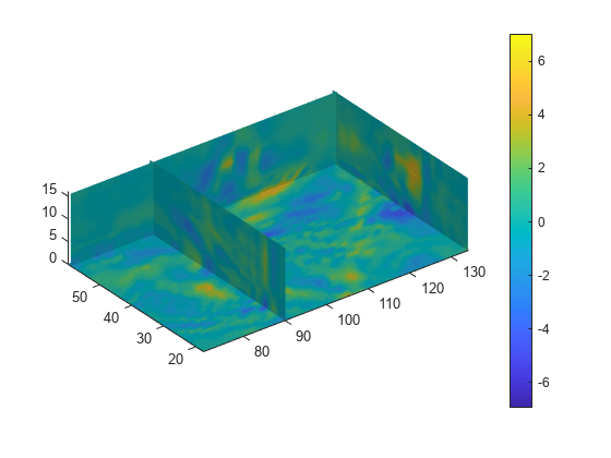
Display the divergence of vector volume data as slice planes. Show the divergence at the yz-planes with x=90 and x=134, at the xz-plane with y=59, and at the xy-plane with z=0. Use color to indicate divergence.

h = slice(x,y,z,div,[90 134],59,0);
shading interp
colorbar
daspect([1 1 1]);
axis tight
camlight
set([h(1),h(2)],'ambientstrength',0.6);

Figure contains an axes object. The axes object contains 4 objects of type surface.

Specify 2-D coordinates and a vector field.

[x,y] = meshgrid(-8:2:8,-8:2:8);
Fx = 200 - (x.^2 + y.^2);
Fy = 200 - (x.^2 + y.^2);

Plot the vector field components Fx and Fy.

quiver(x,y,Fx,Fy)

Figure contains an axes object. The axes object contains an object of type quiver.

Find the numerical divergence of the 2-D vector field. Plot the contour of the divergence.

D = divergence(x,y,Fx,Fy);
hold on
contour(x,y,D,'ShowText','on')

Figure contains an axes object. The axes object contains 2 objects of type quiver, contour.

Input Arguments

collapse all

Input coordinates, specified as matrices or 3-D arrays.

  • For 2-D vector fields, X and Y must be 2-D matrices of the same size, and that size can be no smaller than 2-by-2.

  • For 3-D vector fields, X, Y, and Z must be 3-D arrays of the same size, and that size can be no smaller than 2-by-2-by-2.

Data Types: single | double
Complex Number Support: Yes

Vector field components at the input coordinates, specified as matrices or 3-D arrays. Fx, Fy, and Fz must be the same size as X, Y, and Z.

Data Types: single | double
Complex Number Support: Yes

More About

collapse all

Numerical Divergence

The numerical divergence of a vector field is a way to estimate the values of the divergence using the known values of the vector field at certain points.

For a 3-D vector field of three variables F(x,y,z)=Fx(x,y,z)e^x+Fy(x,y,z)e^y+Fz(x,y,z)e^z, the definition of the divergence of F is

div F=·F=Fxx+Fyy+Fzz.

For a 2-D vector field of two variables F(x,y)=Fx(x,y)e^x+Fy(x,y)e^y, the divergence is

div F=·F=Fxx+Fyy.

Algorithms

divergence computes the partial derivatives in its definition by using finite differences. For interior data points, the partial derivatives are calculated using central difference. For data points along the edges, the partial derivatives are calculated using single-sided (forward) difference.

For example, consider a 2-D vector field F that is represented by the matrices Fx and Fy at locations X and Y with size m-by-n. The locations are 2-D grids created by [X,Y] = meshgrid(x,y), where x is a vector of length n and y is a vector of length m. divergence then computes the partial derivatives Fx / ∂x and Fy / ∂y as

  • dFx(:,i) = (Fx(:,i+1) - Fx(:,i-1))/(x(i+1) - x(i-1)) and

    dFy(j,:) = (Fy(j+1,:) - Fy(j-1,:))/(y(j+1) - y(j-1))

    for interior data points.

  • dFx(:,1) = (Fx(:,2) - Fx(:,1))/(x(2) - x(1)) and

    dFx(:,n) = (Fx(:,n) - Fx(:,n-1))/(x(n) - x(n-1))

    for data points at the left and right edges.

  • dFy(1,:) = (Fy(2,:) - Fy(1,:))/(y(2) - y(1)) and

    dFy(m,:) = (Fy(m,:) - Fy(m-1,:))/(y(m) - y(m-1))

    for data points at the top and bottom edges.

The numerical divergence of the vector field is equal to div = dFx + dFy.

Extended Capabilities

Version History

Introduced before R2006a
Go to top of page