Colorize Aerial Point Cloud Using Aerial Image

Since R2025a

This example shows how to use the coordinate reference system (CRS) information to fuse the color from aerial imagery onto aerial point cloud data.

Merging aerial imagery with an aerial point cloud enhances the visualization and analysis of the point cloud. Combining surface textures with a point cloud can enable you to perform feature extraction and object recognition, as well as help you create digital twins.

Load Aerial Point Cloud Data and Extract CRS Information

Create a lasFileReader object to load the aerial point cloud data from the LAZ file aerialLidarData.laz. The data has been obtained from an OpenTopography data set [1].

pcfile = fullfile(toolboxdir("lidar"),"lidardata","las","aerialLidarData.laz");
lasReader = lasFileReader(pcfile);

Read the point cloud data from the LAZ file using the readPointCloud object function.

pc = readPointCloud(lasReader); 

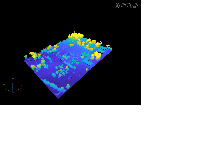
Visualize the point cloud using the pcviewer function.

pcviewer(pc)

Read the CRS data from the LAZ file using the readCRS object function. In this example, the function returns a projected CRS object, which provides information to assign Cartesian x- and y-coordinates to physical locations.

crs = readCRS(lasReader);

Load Aerial Image

This example uses an aerial image obtained by U.S. Geological Survey (USGS) Earth Resources Observation and Science (EROS) Center as a part of National Agriculture Imagery Program (NAIP) [2]. Import the image along with spatial referencing information using the readgeoraster (Mapping Toolbox) function.

[satImg,satSpatialRef] = readgeoraster("m_3308742_se_16_1_20090621_cropped.tif");

Visualize the image using the mapshow (Mapping Toolbox) function.

mapshow(satImg,satSpatialRef)
axis off

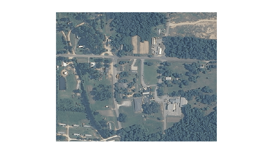
Fuse Color Information from Aerial Image onto Aerial Point Cloud

To fuse color information from image onto point cloud, you must verify that their CRSs are the same using the isequal (Mapping Toolbox) function. If CRSs are different, transform the coordinates from one projected CRS to the other. For more information, see Transform Coordinates to a Different Projected CRS (Mapping Toolbox).

if isequal(crs,satSpatialRef.ProjectedCRS)
    xloc = pc.Location(:,1);
    yloc = pc.Location(:,2);
else
    % Transform the Cartesian coordinates of the point cloud to latitude-longitude coordinates
    [lat,lon] = projinv(crs,pc.Location(:,1),pc.Location(:,2));

    % Transform the latitude-longitude coordinates to image coordinates
    [xloc,yloc] = projfwd(satSpatialRef.ProjectedCRS,lat,lon);
end

Transform the image coordinates to pixel indices using the worldToDiscrete (Mapping Toolbox) function.

[xIdx,yIdx] = worldToDiscrete(satSpatialRef,xloc,yloc); 

Calculate the linear indices to create a one-to-one correspondence between each point in the point cloud and a pixel in the image.

% Identify non-NaN indices
nonNanIdx = ~(isnan(xIdx)|isnan(yIdx));

% Calculate the linear indices
idx = sub2ind(size(satImg,[1 2]),xIdx(nonNanIdx),yIdx(nonNanIdx));

% Calculate the linear indices for each color channel
numImgPixels = prod(size(satImg,[1 2]));
rgbIdx = idx + (0:2)*numImgPixels;

Assign the color from the image to the point cloud data using the calculated indices.

color = zeros(pc.Count,3,"uint8");
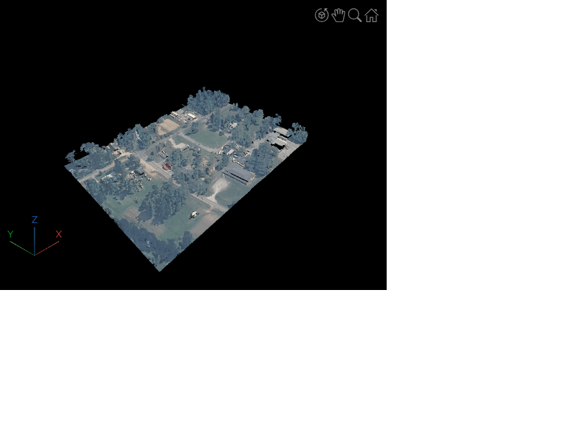
color(nonNanIdx,:) = satImg(rgbIdx);

Visualize the colorized point cloud using the pcviewer function.

pcviewer(pc,color)

References

[1] OpenTopography. "Tuscaloosa, AL: Seasonal Inundation Dynamics And Invertebrate Communities." OpenTopography, 2011. https://doi.org/10.5069/G9SF2T3K.

[2] Earth Resources Observation And Science (EROS) Center. "National Agriculture Imagery Program (NAIP)." Tiff. U.S. Geological Survey, 2017. https://doi.org/10.5066/F7QN651G.