watershed
Watershed transform
Description
The watershed transform finds "catchment basins" or "watershed ridge lines" in an image by treating it as a surface where light pixels represent high elevations and dark pixels represent low elevations. The watershed transform can be used to segment contiguous regions of interest into distinct objects.
Examples
Create a binary image containing two overlapping circular objects. Display the image.
center1 = -40;
center2 = -center1;
dist = sqrt(2*(2*center1)^2);
radius = dist/2 * 1.4;
lims = [floor(center1-1.2*radius) ceil(center2+1.2*radius)];
[x,y] = meshgrid(lims(1):lims(2));
bw1 = sqrt((x-center1).^2 + (y-center1).^2) <= radius;
bw2 = sqrt((x-center2).^2 + (y-center2).^2) <= radius;
bw = bw1 | bw2;
imshow(bw)
title('Binary Image with Overlapping Objects')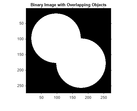
Calculate the distance transform of the complement of the binary image. The value of each pixel in the output image is the distance between that pixel and the nearest nonzero pixel of bw.
D = bwdist(~bw);
imshow(D,[])
title('Distance Transform of Binary Image')
Take the complement of the distance transformed image so that light pixels represent high elevations and dark pixels represent low elevations for the watershed transform.
D = -D;
imshow(D,[])
title('Complement of Distance Transform')
Calculate the watershed transform. Set pixels that are outside the ROI to 0.
L = watershed(D);
L(~bw) = 0;
Display the resulting label matrix as an RGB image.
rgb = label2rgb(L,'jet',[.5 .5 .5]);
imshow(rgb)
title('Watershed Transform')

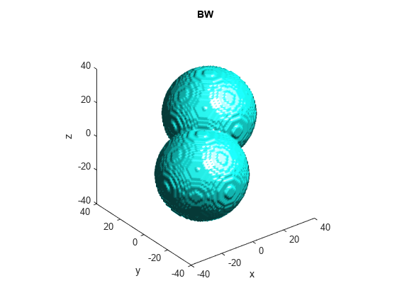
Make a 3-D binary image containing two overlapping spheres.
center1 = -10;
center2 = -center1;
dist = sqrt(3*(2*center1)^2);
radius = dist/2 * 1.4;
lims = [floor(center1-1.2*radius) ceil(center2+1.2*radius)];
[x,y,z] = meshgrid(lims(1):lims(2));
bw1 = sqrt((x-center1).^2 + (y-center1).^2 + ...
           (z-center1).^2) <= radius;
bw2 = sqrt((x-center2).^2 + (y-center2).^2 + ...
           (z-center2).^2) <= radius;
bw = bw1 | bw2;
figure, isosurface(x,y,z,bw,0.5), axis equal, title('BW')
xlabel x, ylabel y, zlabel z
xlim(lims), ylim(lims), zlim(lims)
view(3), camlight, lighting gouraud
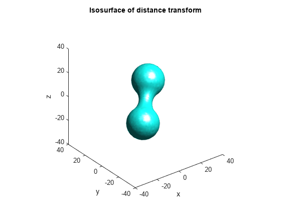
Compute the distance transform.
D = bwdist(~bw);
figure, isosurface(x,y,z,D,radius/2), axis equal
title('Isosurface of distance transform')
xlabel x, ylabel y, zlabel z
xlim(lims), ylim(lims), zlim(lims)
view(3), camlight, lighting gouraud
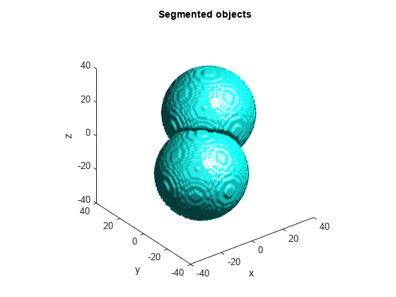
Complement the distance transform, force nonobject pixels to be Inf, and then compute the watershed transform.
D = -D;
D(~bw) = Inf;
L = watershed(D);
L(~bw) = 0;
figure
isosurface(x,y,z,L==1,0.5)
isosurface(x,y,z,L==2,0.5)
axis equal
title('Segmented objects')
xlabel x, ylabel y, zlabel z
xlim(lims), ylim(lims), zlim(lims)
view(3), camlight, lighting gouraud
You can suppress shallow regional minima to avoid oversegmentation during watershed segmentation.
Load an RGB image of pears to segment. Convert the image to grayscale and display it. The center of each pear is bright, corresponding to a regional maximum.
RGB = imread("pears.png");
I = im2gray(RGB);
imshow(I)
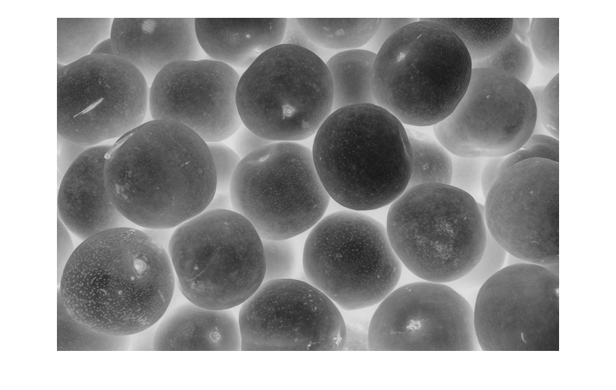
In watershed segmentation, the image is analogous to a surface comprised of watershed lines and catchment basins. When water flows into the surface, it pools in the catchment basins. In a grayscale image, local minima are the catchment basins. To segment the pears, invert the image so the centers of the pears become regional minima.
Icomp = imcomplement(I);
imshow(Icomp)
Display the inverted image as a 3-D surface, in which the third dimension for each pixel is its intensity value. The deeper regions for each pear have spiky bottoms, indicating many shallow regional minima, like catchment basins into which water can pool.
surf(Icomp,EdgeColor="none")
colormap(gray)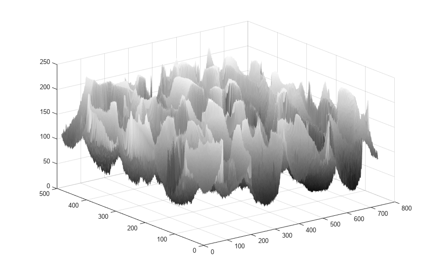
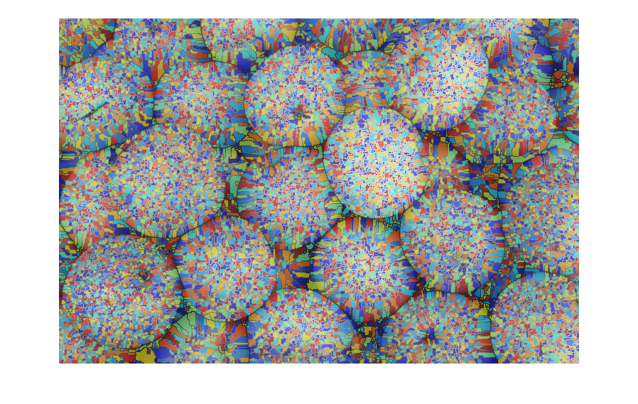
Segment the unfiltered image and display the result as a label overlay. The image is oversegmented, meaning there are many small masks rather than one mask for each pear.
L = watershed(Icomp);
overlay = labeloverlay(I,L);
imshow(overlay)
Suppress the shallow minima by applying the H-minima transform. The value for h has been determined by using trial and error. Change the value to see how the h value affects the segmentation result.
h = 30;
Ifilt = imhmin(Icomp,h);
30;
Ifilt = imhmin(Icomp,h);Display the filtered image as a 3-D surface.
surf(Ifilt,EdgeColor="none")
colormap(gray)
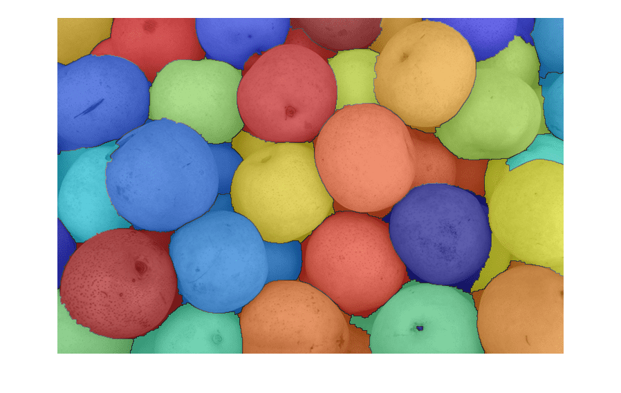
Segment the filtered image and display the result. The image contains approximately one mask for each pear in the foreground.
Lfilt = watershed(Ifilt);
overlayfilt = labeloverlay(I,Lfilt);
imshow(overlayfilt)
Input Arguments
Input image, specified as a numeric or logical array of any dimension.
Data Types: single | double | int8 | int16 | int32 | int64 | uint8 | uint16 | uint32 | uint64 | logical
Pixel connectivity, specified as one of the values in this table. The
default connectivity is 8 for 2-D images, and
26 for 3-D images.
Value | Meaning | |
|---|---|---|
Two-Dimensional Connectivities | ||
| Pixels are connected if their edges touch. The neighborhood of a pixel are the adjacent pixels in the horizontal or vertical direction. |
Current pixel is shown in gray. |
| Pixels are connected if their edges or corners touch. The neighborhood of a pixel are the adjacent pixels in the horizontal, vertical, or diagonal direction. |
Current pixel is shown in gray. |
Three-Dimensional Connectivities | ||
| Pixels are connected if their faces touch. The neighborhood of a pixel are the adjacent pixels in:
|
Current pixel is shown in gray. |
| Pixels are connected if their faces or edges touch. The neighborhood of a pixel are the adjacent pixels in:
|
Current pixel is center of cube. |
| Pixels are connected if their faces, edges, or corners touch. The neighborhood of a pixel are the adjacent pixels in:
|
Current pixel is center of cube. |
For higher dimensions, watershed uses the default value
conndef(ndims(A),"maximal")
Connectivity can also be
defined in a more general way for any dimension by specifying a 3-by-3-by- ... -by-3 matrix of
0s and 1s. The 1-valued elements
define neighborhood locations relative to the center element of conn. Note
that conn must be symmetric about its center element. See Specifying Custom Connectivities for more information.
Note
If you specify a nondefault connectivity, then pixels on the edge of
the image might not be considered to be border pixels. For example, if
conn = [0 0 0; 1 1 1; 0 0 0], elements on the
first and last row are not considered to be border pixels because,
according to that connectivity definition, they are not connected to the
region outside the image.
Data Types: double | logical
Output Arguments
Label matrix, specified as a numeric array of nonnegative integers. The elements labeled
0 do not belong to a unique watershed region. The
elements labeled 1 belong to the first watershed region,
the elements labeled 2 belong to the second watershed region, and so
on.
Tips
To prevent oversegmentation, remove shallow minima from the image by using the
imhminfunction before you use thewatershedfunction.
Algorithms
watershed uses the Fernand Meyer algorithm [1].
References
[1] Meyer, Fernand, "Topographic distance and watershed lines,” Signal Processing , Vol. 38, July 1994, pp. 113-125.
Extended Capabilities
Usage notes and limitations:
watershedsupports the generation of C code (requires MATLAB® Coder™). Note that if you choose the genericMATLAB Host Computertarget platform,watershedgenerates code that uses a precompiled, platform-specific shared library. Use of a shared library preserves performance optimizations but limits the target platforms for which code can be generated. For more information, see Types of Code Generation Support in Image Processing Toolbox.Supports only 2-D images
Supports only
4or8connectivitySupports images containing up to 65,535 regions
Output type is always
uint16
Usage notes and limitations:
Supports only 2-D images
Supports only
4or8connectivitySupports images containing up to 65,535 regions
Output type is always
uint16
This function fully supports thread-based environments. For more information, see Run MATLAB Functions in Thread-Based Environment.
Version History
Introduced before R2006awatershed now supports thread-based
environments.
MATLAB Command
You clicked a link that corresponds to this MATLAB command:
Run the command by entering it in the MATLAB Command Window. Web browsers do not support MATLAB commands.
Select a Web Site
Choose a web site to get translated content where available and see local events and offers. Based on your location, we recommend that you select: .
You can also select a web site from the following list
How to Get Best Site Performance
Select the China site (in Chinese or English) for best site performance. Other MathWorks country sites are not optimized for visits from your location.
Americas
- América Latina (Español)
- Canada (English)
- United States (English)
Europe
- Belgium (English)
- Denmark (English)
- Deutschland (Deutsch)
- España (Español)
- Finland (English)
- France (Français)
- Ireland (English)
- Italia (Italiano)
- Luxembourg (English)
- Netherlands (English)
- Norway (English)
- Österreich (Deutsch)
- Portugal (English)
- Sweden (English)
- Switzerland
- United Kingdom (English)


