Comparison of Auto White Balance Algorithms

This example shows how to estimate illumination and perform white balance of a scene using three different illumination algorithms. The example compares the estimated illuminant to a ground truth illuminant calculated using an X-Rite® ColorChecker® chart.

Eyes are very good at judging what is white under different lighting conditions. Digital cameras, however, without some kind of adjustment, can easily capture unrealistic images with a strong color cast. Automatic white balance (AWB) algorithms try to correct for the ambient light with minimum input from the user, so that the resulting image looks like what our eyes would see.

Automatic white balancing is done in two steps:

• Step 1: Estimate the scene illuminant.

• Step 2: Correct the color balance of the image.

Several different algorithms exist to estimate scene illuminant. The performance of each algorithm depends on the scene, lighting, and imaging conditions. This example judges the quality of three algorithms for illuminant estimation for one specific image by comparing them to the ground truth scene illuminant:

• White Patch Retinex [1]

• Gray World [2]

• Cheng's Principal Component Analysis (PCA) method [3]

After the ambient light is known, then correcting the colors in the image (Step 2) is an easy and fixed process.

Read and Preprocess Raw Camera Data

AWB algorithms are usually applied on the raw image data after a minimal amount of preprocessing, before the image is compressed and saved to the memory card.

Read a 16-bit raw image into the workspace. foosballraw.tiff is an image file that contains raw sensor data after correcting the black level and scaling the intensities to 16 bits per pixel. This image is free of the white balancing done by the camera, as well as other preprocessing operations such as demosaicing, denoising, chromatic aberration compensation, tone adjustments, and gamma correction.

A = imread('foosballraw.tiff');

Interpolate to Recover Missing Color Information

Digital cameras use a color filter array superimposed on the imaging sensor to simulate color vision, so that each pixel is sensitive to either red, green or blue. To recover the missing color information at every pixel, interpolate using the demosaic function. The Bayer pattern used by the camera with which the photo was captured (Canon EOS 30D) is RGGB.

A = demosaic(A,'rggb');

Gamma-Correct Image for Detection and Display

The image A contains linear RGB values. Linear RGB values are appropriate for estimating scene illuminant and correcting the color balance of an image. However, if you try to display the linear RGB image, it will appear very dim, because of the nonlinear characteristic of display devices. Therefore, for display purposes, gamma-correct the image to the sRGB color space using the lin2rgb function.

A_sRGB = lin2rgb(A);

Display the demosaiced image before and after gamma correction.

montage({A,A_sRGB})
title('Original Image Before and After Gamma Correction')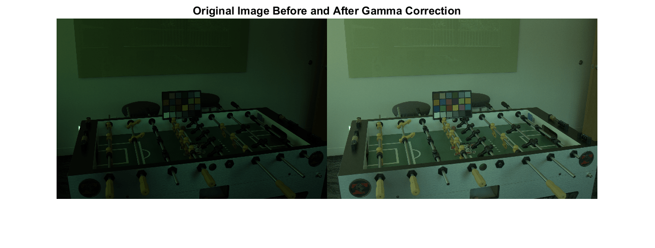

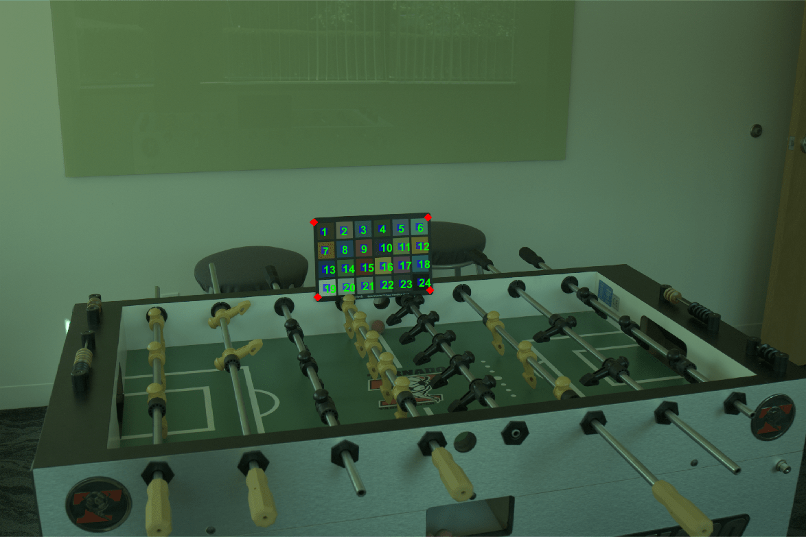
Measure Ground Truth Illuminant Using ColorChecker Chart

Calculate the ground truth illuminant using the X-Rite ColorChecker chart that is included in the scene. This chart consists of 24 neutral and color patches with known spectral reflectances.

Detect the chart in the gamma-corrected image by using the colorChecker function. The linear RGB image is too dark for colorChecker to detect the chart automatically.

chart_sRGB = colorChecker(A_sRGB);

Confirm that the chart is detected correctly.

displayChart(chart_sRGB)

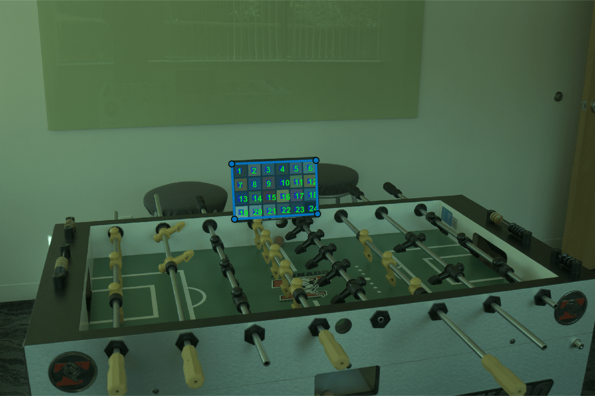
Get the coordinates of the registration points at the four corners of the chart.

registrationPoints = chart_sRGB.RegistrationPoints;

Create a new colorChecker object from the linear RGB data. Specify the location of the chart using the coordinates of the registration points.

chart = colorChecker(A,"RegistrationPoints",registrationPoints);

Measure the ground truth illuminant of the linear RGB data using the measureIlluminant function.

illuminant_groundtruth = measureIlluminant(chart)

illuminant_groundtruth = 1×3
103 ×

    4.5407    9.3226    6.1812

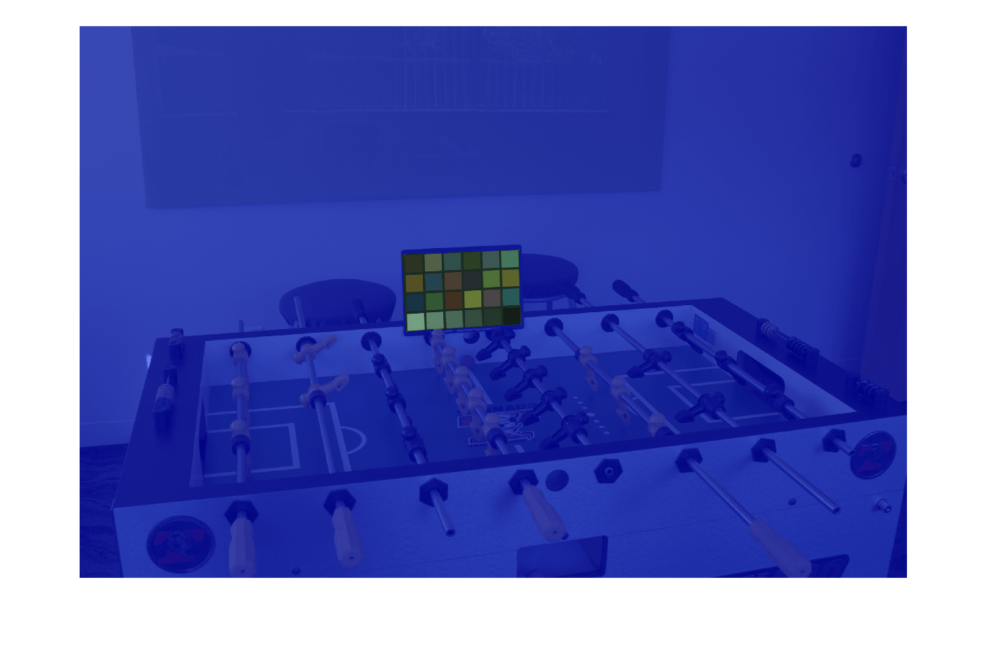
Create Mask of ColorChecker Chart

When testing the AWB algorithms, prevent the algorithms from unfairly taking advantage of the chart by masking out the chart.

Create a polygon ROI over the chart by using the drawpolygon function. Specify the vertices of the polygon as the registration points.

chartROI = drawpolygon("Position",registrationPoints);

Convert the polygon ROI to a binary mask by using the createMask function.

mask_chart = createMask(chartROI);

Invert the mask. Pixels within the chart are excluded from the mask and pixels of the rest of the scene are included in the mask.

mask_scene = ~mask_chart;

To confirm the accuracy of the mask, display the mask over the image. Pixels included in the mask have a blue tint.

imshow(labeloverlay(A_sRGB,mask_scene));

Angular Error

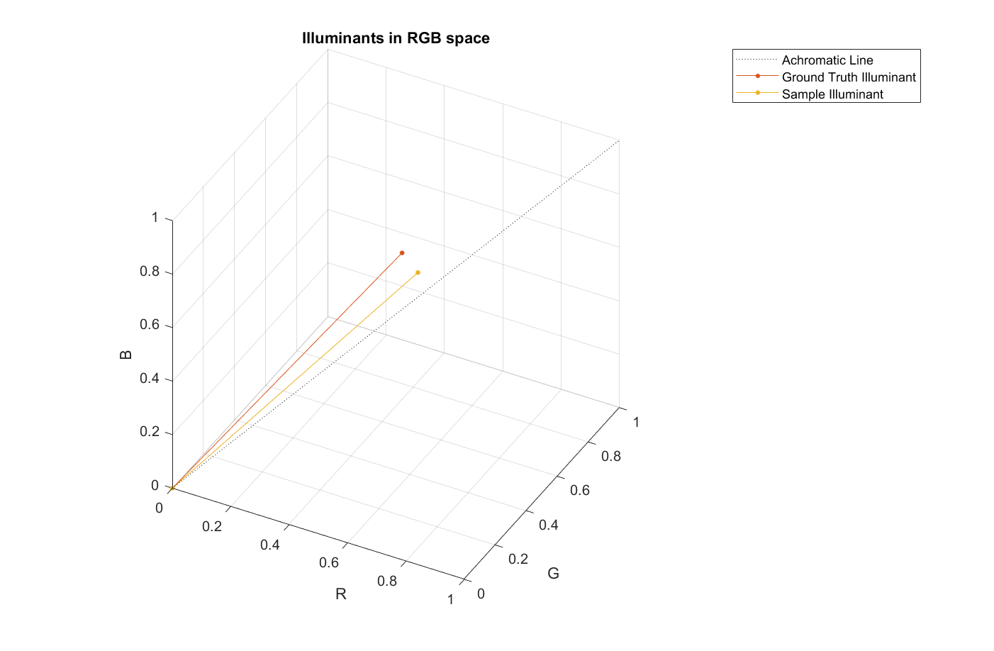
You can consider an illuminant as a vector in 3-D RGB color space. The magnitude of the estimated illuminant does not matter as much as its direction, because the direction of the illuminant is what is used to white balance an image.

To evaluate the quality of an estimated illuminant, compute the angular error between the estimated illuminant and the ground truth. Angular error is the angle (in degrees) formed by the two vectors. The smaller the angular error, the better the estimation is.

To better understand the concept of angular error, consider the following visualization of an arbitrary illuminant and the ground truth measured using the ColorChecker chart. The plotColorAngle helper function plots a unit vector of an illuminant in 3-D RGB color space, and is defined at the end of the example.

sample_illuminant = [0.066 0.1262 0.0691];

p = plot3([0 1],[0 1],[0,1],'LineStyle',':','Color','k');
ax = p.Parent;
hold on
plotColorAngle(illuminant_groundtruth,ax)
plotColorAngle(sample_illuminant,ax)
title('Illuminants in RGB space')  
view(28,36)
legend('Achromatic Line','Ground Truth Illuminant','Sample Illuminant')
grid on
axis equal

White Patch Retinex

The White Patch Retinex algorithm for illuminant estimation assumes that the scene contains a bright achromatic patch. This patch reflects the maximum light possible for each color band, which is the color of the scene illuminant. Use the illumwhite function to estimate illumination using the White Patch Retinex algorithm.

Include All Scene Pixels

Estimate the illuminant using all the pixels in the scene. Exclude the ColorChecker chart from the scene by using the 'Mask' name-value pair argument.

percentileToExclude = 0;
illuminant_wp1 = illumwhite(A,percentileToExclude,'Mask',mask_scene);

Compute the angular error for the illuminant estimated with White Patch Retinex.

err_wp1 = colorangle(illuminant_wp1, illuminant_groundtruth);
disp(['Angular error for White Patch with percentile=0: ' num2str(err_wp1)])

Angular error for White Patch with percentile=0: 16.5381

White balance the image using the chromadapt function. Specify the estimated illuminant and indicate that color values are in the linear RGB color space.

B_wp1 = chromadapt(A,illuminant_wp1,'ColorSpace','linear-rgb');

Display the gamma-corrected white-balanced image.

B_wp1_sRGB = lin2rgb(B_wp1);

figure
imshow(B_wp1_sRGB)
title('White-Balanced Image using White Patch Retinex with percentile=0')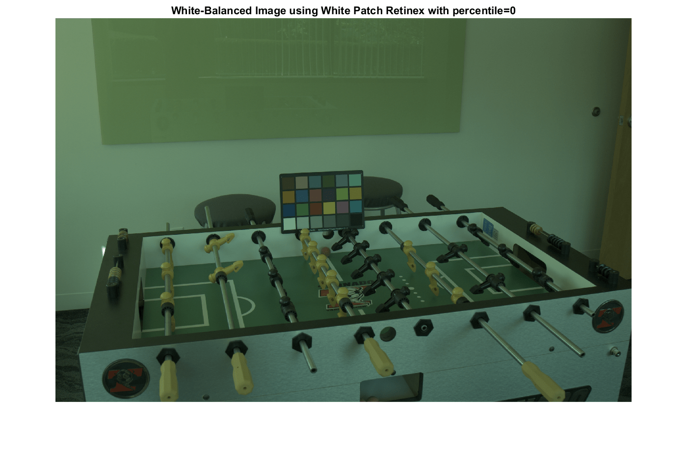

Exclude Brightest Pixels

The White Patch Retinex algorithm does not perform well when pixels are overexposed. To improve the performance of the algorithm, exclude the top 1% of the brightest pixels.

percentileToExclude = 1;
illuminant_wp2 = illumwhite(A,percentileToExclude,'Mask',mask_scene);

Calculate the angular error for the estimated illuminant. The error is less than when estimating the illuminant using all pixels.

err_wp2 = colorangle(illuminant_wp2,illuminant_groundtruth);
disp(['Angular error for White Patch with percentile=1: ' num2str(err_wp2)])

Angular error for White Patch with percentile=1: 5.0324

White balance the image in the linear RGB color space using the estimated illuminant.

B_wp2 = chromadapt(A,illuminant_wp2,'ColorSpace','linear-rgb');

Display the gamma-corrected white-balanced image with the new illuminant.

B_wp2_sRGB = lin2rgb(B_wp2);
imshow(B_wp2_sRGB)
title('White-Balanced Image using White Patch Retinex with percentile=1')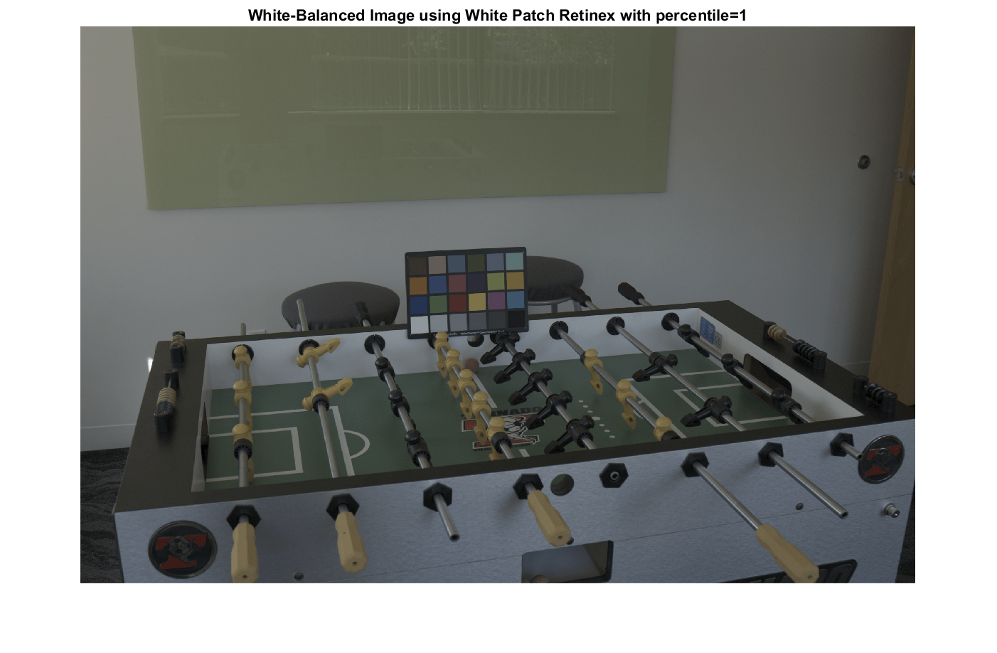

Gray World

The Gray World algorithm for illuminant estimation assumes that the average color of the world is gray, or achromatic. Therefore, it calculates the scene illuminant as the average RGB value in the image. Use the illumgray function to estimate illumination using the Gray World algorithm.

Include All Scene Pixels

First, estimate the scene illuminant using all pixels of the image, excluding those corresponding to the ColorChecker chart. The illumgray function provides a parameter to specify the percentiles of bottom and top values (ordered by brightness) to exclude. Here, specify the percentiles as 0.

percentileToExclude = 0;
illuminant_gw1 = illumgray(A,percentileToExclude,'Mask',mask_scene);

Calculate the angular error between the estimated illuminant and the ground truth illuminant.

err_gw1 = colorangle(illuminant_gw1,illuminant_groundtruth);
disp(['Angular error for Gray World with percentiles=[0 0]: ' num2str(err_gw1)])

Angular error for Gray World with percentiles=[0 0]: 5.0416

White balance the image in the linear RGB color space using the estimated illuminant.

B_gw1 = chromadapt(A,illuminant_gw1,'ColorSpace','linear-rgb');

Display the gamma-corrected white-balanced image.

B_gw1_sRGB = lin2rgb(B_gw1);
imshow(B_gw1_sRGB)
title('White-Balanced Image using Gray World with percentiles=[0 0]')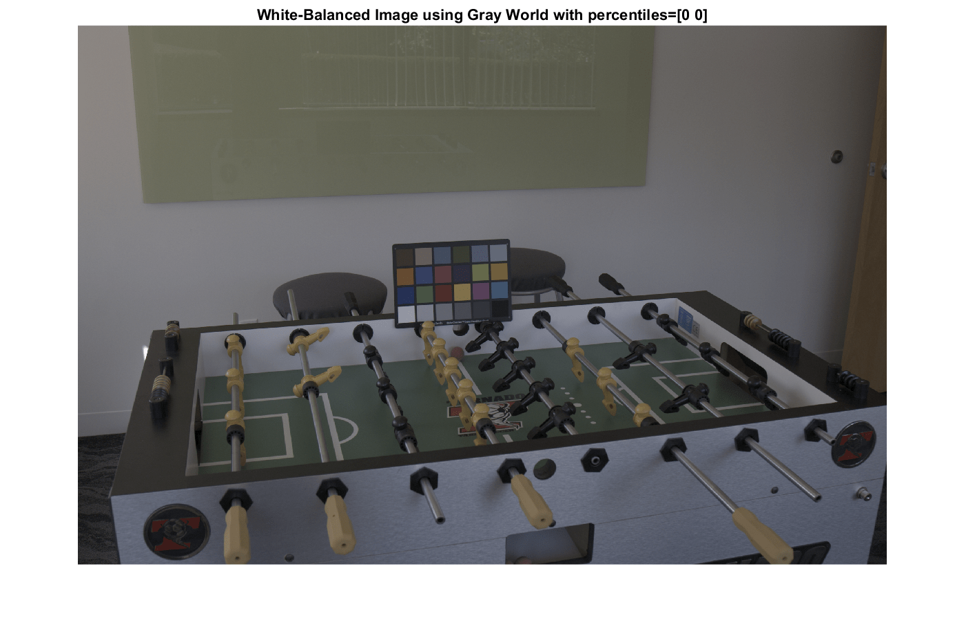

Exclude Brightest and Darkest Pixels

The Gray World algorithm does not perform well when pixels are underexposed or overexposed. To improve the performance of the algorithm, exclude the top 1% of the darkest and brightest pixels.

percentileToExclude = 1;
illuminant_gw2 = illumgray(A,percentileToExclude,'Mask',mask_scene);

Calculate the angular error for the estimated illuminant. The error is less than when estimating the illuminant using all pixels.

err_gw2 = colorangle(illuminant_gw2, illuminant_groundtruth);
disp(['Angular error for Gray World with percentiles=[1 1]: ' num2str(err_gw2)])

Angular error for Gray World with percentiles=[1 1]: 5.1094

White balance the image in the linear RGB color space using the estimated illuminant.

B_gw2 = chromadapt(A,illuminant_gw2,'ColorSpace','linear-rgb');

Display the gamma-corrected white-balanced image with the new illuminant.

B_gw2_sRGB = lin2rgb(B_gw2);
imshow(B_gw2_sRGB)
title('White-Balanced Image using Gray World with percentiles=[1 1]')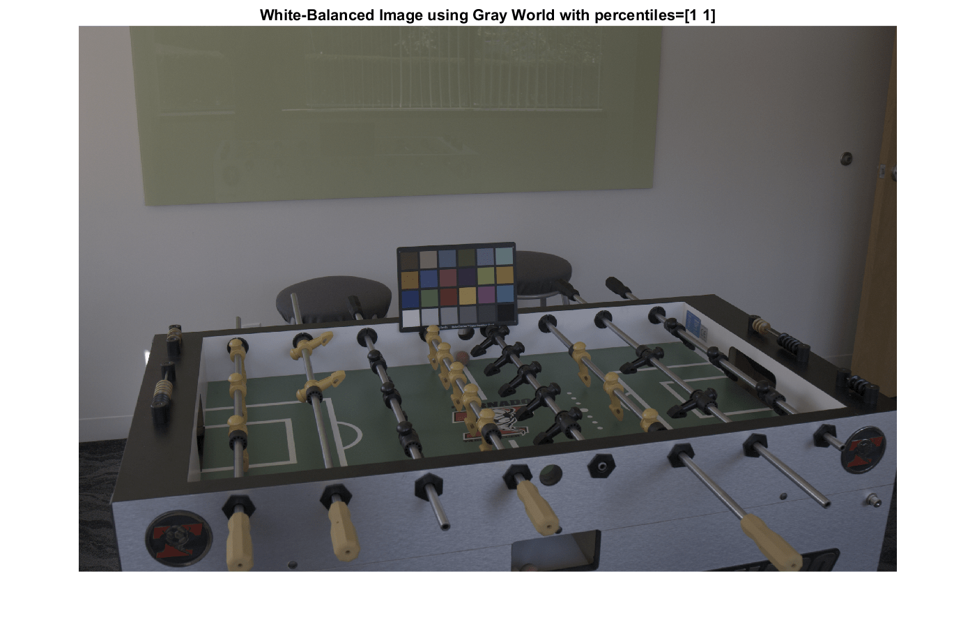

Cheng's Principal Component Analysis (PCA) Method

Cheng's illuminant estimation method draws inspiration from spatial domain methods such as Grey Edge [4], which assumes that the gradients of an image are achromatic. They show that Grey Edge can be improved by artificially introducing strong gradients by shuffling image blocks, and conclude that the strongest gradients follow the direction of the illuminant. Their method consists in ordering pixels according to the norm of their projection along the direction of the mean image color, and retaining the bottom and top percentile. These two groups correspond to strong gradients in the image. Finally, they perform a principal component analysis (PCA) on the retained pixels and return the first component as the estimated illuminant. Use the illumpca function to estimate illumination using Cheng's PCA algorithm.

Include Default Bottom and Top 3.5 Percent of Pixels

First, estimate the illuminant using the default percentage value of Cheng's PCA method, excluding those corresponding to the ColorChecker chart.

illuminant_ch2 = illumpca(A,'Mask',mask_scene);

Calculate the angular error between the estimated illuminant and the ground truth illuminant.

err_ch2 = colorangle(illuminant_ch2,illuminant_groundtruth);
disp(['Angular error for Cheng with percentage=3.5: ' num2str(err_ch2)])

Angular error for Cheng with percentage=3.5: 5.0162

White balance the image in the linear RGB color space using the estimated illuminant.

B_ch2 = chromadapt(A,illuminant_ch2,'ColorSpace','linear-rgb');

Display the gamma-corrected white-balanced image.

B_ch2_sRGB = lin2rgb(B_ch2);
imshow(B_ch2_sRGB)
title('White-Balanced Image using Cheng with percentile=3.5')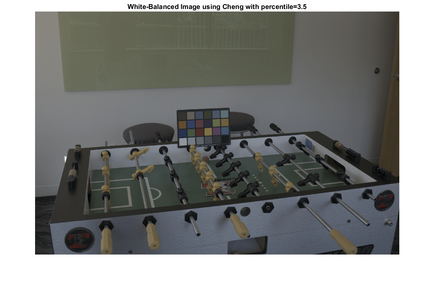

Include Bottom and Top 5 Percent of Pixels

Now, estimate the scene illuminant using the bottom and top 5% of pixels along the direction of the mean color. The second argument of the illumpca function specifies the percentiles of bottom and top values (ordered by brightness) to exclude.

illuminant_ch1 = illumpca(A,5,'Mask',mask_scene);

Calculate the angular error between the estimated illuminant and the ground truth illuminant. The error is less than when estimating the illuminant using the default percentage.

err_ch1 = colorangle(illuminant_ch1, illuminant_groundtruth);
disp(['Angular error for Cheng with percentage=5: ' num2str(err_ch1)])

Angular error for Cheng with percentage=5: 4.7454

White balance the image in the linear RGB color space using the estimated illuminant.

B_ch1 = chromadapt(A,illuminant_ch1,'ColorSpace','linear-rgb');

Display the gamma-corrected white-balanced image.

B_ch1_sRGB = lin2rgb(B_ch1);
imshow(B_ch1_sRGB)
title('White-Balanced Image using Cheng with percentage=5')

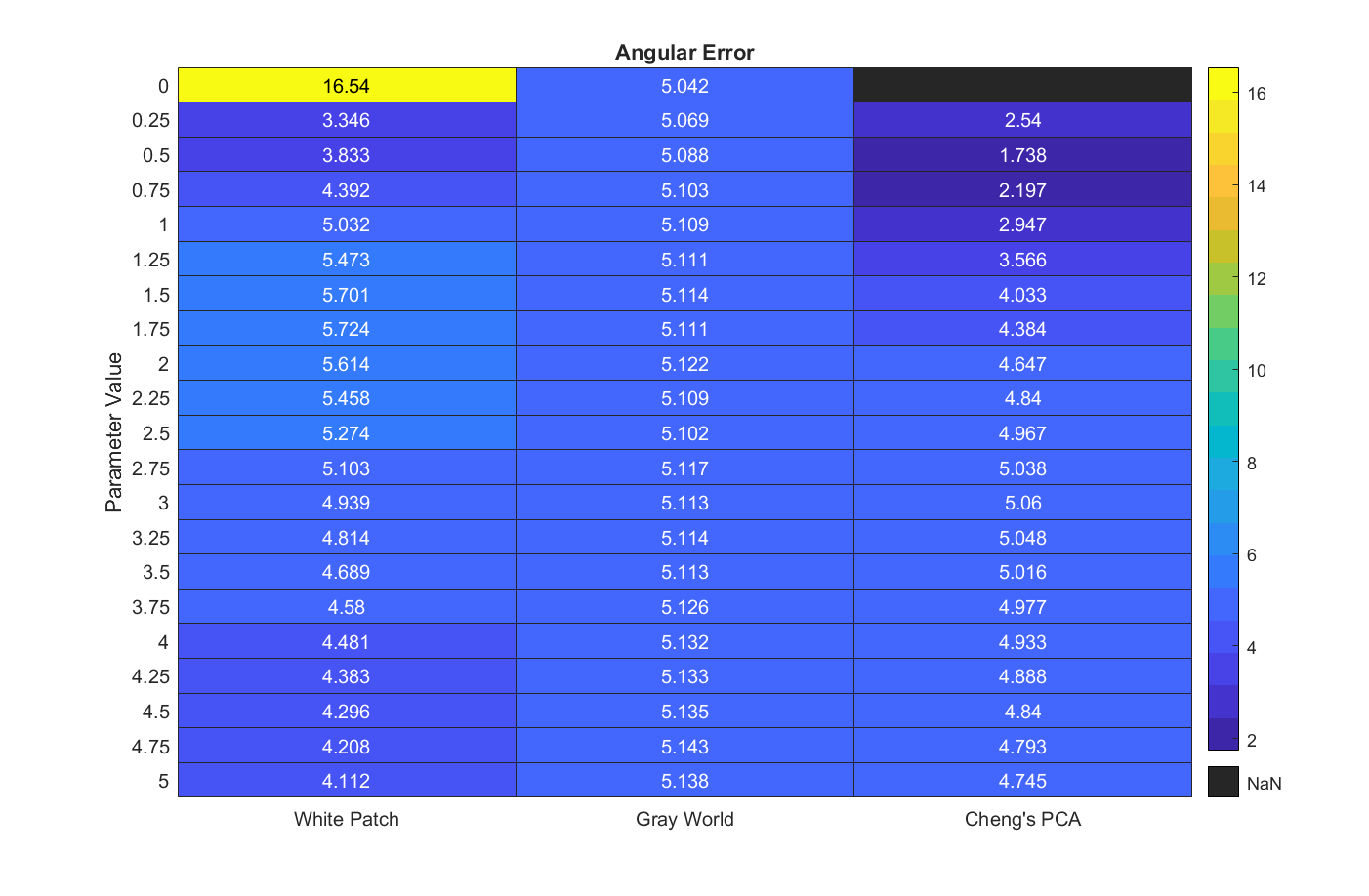
Find Optimal Parameters

To find the best parameter to use for each algorithm, you can sweep through a range and calculate the angular error for each of them. The parameters of the three algorithms have different meanings, but the similar ranges of these parameters makes it easy to programmatically search for the best one for each algorithm.

param_range = 0:0.25:5;
err = zeros(numel(param_range),3);
for k = 1:numel(param_range)
    % White Patch
    illuminant_wp = illumwhite(A,param_range(k),'Mask',mask_scene);
    err(k,1) = colorangle(illuminant_wp,illuminant_groundtruth);
    % Gray World
    illuminant_gw = illumgray(A,param_range(k),'Mask',mask_scene);
    err(k,2) = colorangle(illuminant_gw,illuminant_groundtruth);
    % Cheng
    if (param_range(k) ~= 0)
        illuminant_ch = illumpca(A,param_range(k),'Mask',mask_scene);
        err(k,3) = colorangle(illuminant_ch,illuminant_groundtruth);
    else
        % Cheng's algorithm is undefined for percentage=0.
        err(k,3) = NaN;
    end
end

Display a heatmap of the angular error using the heatmap function. Dark blue colors indicate a low angular error while yellow colors indicate a high angular error. The optimal parameter has the smallest angular error.

heatmap(err,'Title','Angular Error','Colormap',parula(length(param_range)), ...
    'XData',["White Patch" "Gray World" "Cheng's PCA"], ...
    'YLabel','Parameter Value','YData',string(param_range));

Find the best parameter for each algorithm.

[~,idx_best] = min(err);
best_param_wp = param_range(idx_best(1));
best_param_gw = param_range(idx_best(2));
best_param_ch = param_range(idx_best(3));

fprintf('The best parameter for White Patch is %1.2f with angular error %1.2f degrees\n', ...
    best_param_wp,err(idx_best(1),1));

The best parameter for White Patch is 0.25 with angular error 3.35 degrees

fprintf('The best parameter for Gray World is %1.2f with angular error %1.2f degrees\n', ...
    best_param_gw,err(idx_best(2),2));

The best parameter for Gray World is 0.00 with angular error 5.04 degrees

fprintf('The best parameter for Cheng is %1.2f with angular error %1.2f degrees\n', ...
    best_param_ch,err(idx_best(3),3));

The best parameter for Cheng is 0.50 with angular error 1.74 degrees

Calculate the estimated illuminant for each algorithm using the best parameter.

best_illum_wp = illumwhite(A,best_param_wp,'Mask',mask_scene);
best_illum_gw = illumgray(A,best_param_gw,'Mask',mask_scene);
best_illum_ch = illumpca(A,best_param_ch,'Mask',mask_scene);

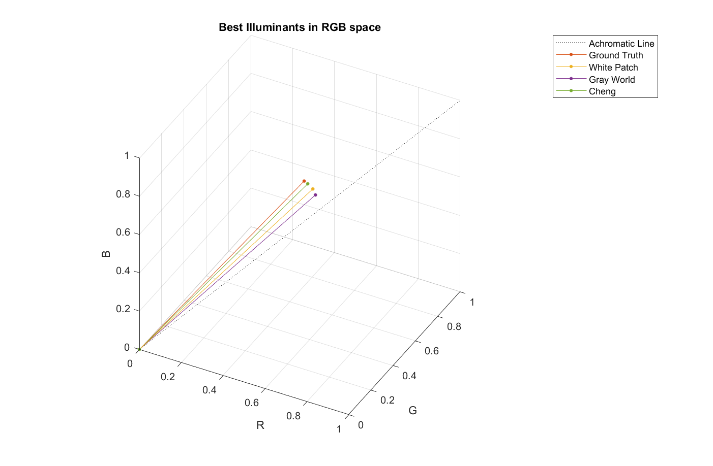
Display the angular error of each best illuminant in the RGB color space.

p = plot3([0 1],[0 1],[0,1],'LineStyle',':','Color','k');
ax = p.Parent;
hold on
plotColorAngle(illuminant_groundtruth,ax)
plotColorAngle(best_illum_wp,ax)
plotColorAngle(best_illum_gw,ax)
plotColorAngle(best_illum_ch,ax)
title('Best Illuminants in RGB space')
view(28,36)
legend('Achromatic Line','Ground Truth','White Patch','Gray World','Cheng')
grid on
axis equal

Calculate the optimal white-balanced images for each algorithm using the best illuminant.

B_wp_best = chromadapt(A,best_illum_wp,'ColorSpace','linear-rgb');
B_wp_best_sRGB = lin2rgb(B_wp_best);
B_gw_best = chromadapt(A,best_illum_gw,'ColorSpace','linear-rgb');
B_gw_best_sRGB = lin2rgb(B_gw_best);
B_ch_best = chromadapt(A,best_illum_ch,'ColorSpace','linear-rgb');
B_ch_best_sRGB = lin2rgb(B_ch_best);

Display the optimal white-balanced images for each algorithm in a montage.

figure
montage({B_wp_best_sRGB,B_gw_best_sRGB,B_ch_best_sRGB},'Size',[1 3])
title('Montage of Best White-Balanced Images: White Point, Gray World, Cheng')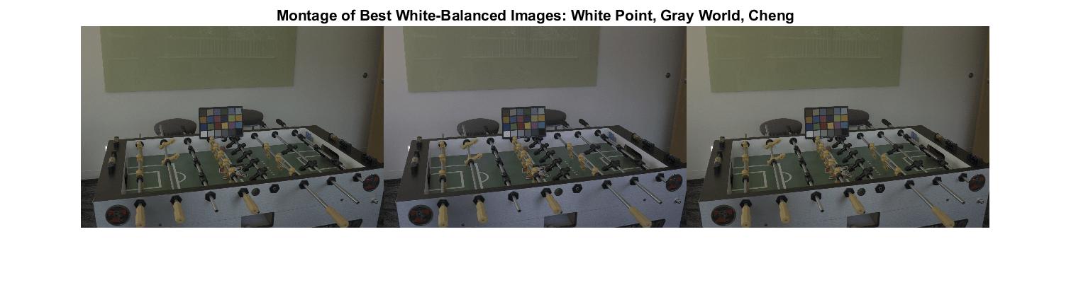

Conclusion

This comparison of two classic illuminant estimation algorithms and a more recent one shows that Cheng's method, using the top and bottom 0.75% darkest and brightest pixels, wins for that particular image. However, this result should be taken with a grain of salt.

First, the ground truth illuminant was measured using a ColorChecker chart and is sensitive to shot and sensor noise. The ground truth illuminant of a scene can be better estimated using a spectrophotometer.

Second, the ground truth illuminant is estimated as the mean color of the neutral patches. It is common to use the median instead of the mean, which could shift the ground truth by a significant amount. For example, for the image in this study, using the same pixels, the median color and the mean color of the neutral patches are 0.5 degrees apart, which in some cases can be more than the angular error of the illuminants estimated by different algorithms.

Third, a full comparison of illuminant estimation algorithms should use a variety of images taken under different conditions. One algorithm might work better than the others for a particular image, but might perform poorly over the entire data set.

Supporting Function

The plotColorAngle function plots a unit vector of an illuminant in 3-D RGB color space. The input argument illum specifies the illuminant as an RGB color and the input argument ax specifies the axes on which to plot the unit vector.

function plotColorAngle(illum,ax)
    R = illum(1);
    G = illum(2);
    B = illum(3);
    magRGB = norm(illum);
    plot3([0 R/magRGB],[0 G/magRGB],[0 B/magRGB], ...
        'Marker','.','MarkerSize',10,'Parent',ax)
    xlabel('R')
    ylabel('G')
    zlabel('B')
    xlim([0 1])
    ylim([0 1])
    zlim([0 1])
end

References

[1] Ebner, Marc. White Patch Retinex, Color Constancy. John Wiley & Sons, 2007. ISBN 978-0-470-05829-9.

[2] Ebner, Marc. The Gray World Assumption, Color Constancy. John Wiley & Sons, 2007. ISBN 978-0-470-05829-9.

[3] Cheng, Dongliang, Dilip K. Prasad, and Michael S. Brown. "Illuminant estimation for color constancy: why spatial-domain methods work and the role of the color distribution." JOSA A 31.5 (2014): 1049-1058.

[4] Van De Weijer, Joost, Theo Gevers, and Arjan Gijsenij. "Edge-based color constancy." IEEE Transactions on image processing 16.9 (2007): 2207-2214.