Estimate Polynomial Models in the App

 Prerequisites

Before you can perform this task, you must have:

• Imported data into the System Identification app. See Import Time-Domain Data into the App. For supported data formats, see Data Supported by Polynomial Models.

• Performed any required data preprocessing operations. To improve the accuracy of your model, you should detrend your data. Removing offsets and trends is especially important for Output-Error (OE) models and has less impact on the accuracy of models that include a flexible noise model structure, such as ARMAX and Box-Jenkins. See Ways to Prepare Data for System Identification.

• Select a model structure, model orders, and delays. For a list of available structures, see What Are Polynomial Models? For more information about how to estimate model orders and delays, see Estimating Orders and Delays in the App. For multiple-output models, you must specify order matrices in the MATLAB^® workspace, as described in Polynomial Sizes and Orders of Multi-Output Polynomial Models.

1. In the System Identification app, select Estimate > Polynomial Models to open the Polynomial Models dialog box.

   

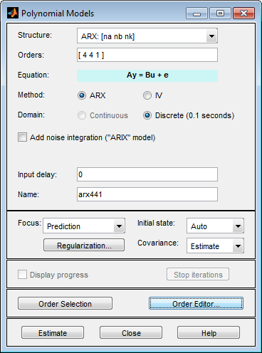
   For more information on the options in the dialog box, click Help.

2. In the Structure list, select the polynomial model structure you want to estimate from the following options:

   • ARX:[na nb nk]

   • ARMAX:[na nb nc nk]

   • OE:[nb nf nk]

   • BJ:[nb nc nd nf nk]

   This action updates the options in the Polynomial Models dialog box to correspond with this model structure. For information about each model structure, see What Are Polynomial Models?.

   Note

   For time-series data, only AR and ARMA models are available. For more information about estimating time-series models, see Time Series Analysis.

3. In the Orders field, specify the model orders and delays, as follows:

   • For single-output polynomial models, enter the model orders and delays according to the sequence displayed in the Structure field. For multiple-input models, specify nb and nk as row vectors with as many elements as there are inputs. If you are estimating BJ and OE models, you must also specify nf as a vector.

     For example, for a three-input system, nb can be [1 2 4], where each element corresponds to an input.

   • For multiple-output models, enter the model orders as described in Polynomial Sizes and Orders of Multi-Output Polynomial Models.

   Tip

   To enter model orders and delays using the Order Editor dialog box, click Order Editor.

4. (ARX models only) Select the estimation Method as ARX or IV (instrumental variable method). For information about the algorithms, see Polynomial Model Estimation Algorithms.

5. (ARX, ARMAX, and BJ models only) Check the Add noise integration check box to add an integrator to the noise source, e.

6. Specify the delay using the Input delay edit box. The value must be a vector of length equal to the number of input channels in the data. For discrete-time estimations (any estimation using data with nonzero sample-time), the delay must be expressed in the number of lags. These delays are separate from the “in-model” delays specified by the nk order in the Orders edit box.

7. In the Name field, edit the name of the model or keep the default.

8. In the Focus list, select how to weigh the relative importance of the fit at different frequencies. For more information about each option, see Assigning Estimation Weightings.

9. In the Initial state list, specify how you want the algorithm to treat initial conditions. For more information about the available options, see Specifying Initial Conditions for Iterative Estimation Algorithms.

   Tip

   If you get an inaccurate fit, try setting a specific method for handling initial states rather than choosing it automatically.

10. In the Covariance list, select Estimate if you want the algorithm to compute parameter uncertainties. Effects of such uncertainties are displayed on plots as model confidence regions.

    To omit estimating uncertainty, select None. Skipping uncertainty computation for large, multiple-output models might reduce computation time.

11. Click Regularization to obtain regularized estimates of model parameters. Specify the regularization constants in the Regularization Options dialog box. To learn more, see Regularized Estimates of Model Parameters.

12. (ARMAX, OE, and BJ models only) To view the estimation progress in the MATLAB Command Window, select the Display progress check box. This launches a progress viewer window in which estimation progress is reported.

13. Click Estimate to add this model to the Model Board in the System Identification app.

14. (Prediction-error method only) To stop the search and save the results after the current iteration has been completed, click Stop Iterations. To continue iterations from the current model, click the Continue iter button to assign current parameter values as initial guesses for the next search.

Assigning Estimation Weightings

You can specify how the estimation algorithm weighs the fit at various frequencies. In the app, set Focus to one of the following options:

• Prediction — Uses the inverse of the noise model H to weigh the relative importance of how closely to fit the data in various frequency ranges. Corresponds to minimizing one-step-ahead prediction, which typically favors the fit over a short time interval. Optimized for output prediction applications.

• Simulation — Uses the input spectrum to weigh the relative importance of the fit in a specific frequency range. Does not use the noise model to weigh the relative importance of how closely to fit the data in various frequency ranges. Optimized for output simulation applications.

• Stability — Estimates the best stable model. For more information about model stability, see Unstable Models.

• Filter — Specify a custom filter to open the Estimation Focus dialog box, where you can enter a filter, as described in Simple Passband Filter or Defining a Custom Filter. This prefiltering applies only for estimating the dynamics from input to output. The disturbance model is determined from the unfiltered estimation data.

Next Steps

• Validate the model by selecting the appropriate check box in the Model Views area of the System Identification app. For more information about validating models, see Validating Models After Estimation.

• Export the model to the MATLAB workspace for further analysis by dragging it to the To Workspace rectangle in the System Identification app.

  Tip

  For ARX and OE models, you can use the exported model for initializing a nonlinear estimation at the command line. This initialization may improve the fit of the model. See Initialize Nonlinear ARX Estimation Using Linear Model, and Initialize Hammerstein-Wiener Estimation Using Linear Model.

Related Examples

• Preliminary Step – Estimating Model Orders and Input Delays
• Estimate Polynomial Models at the Command Line

More About

• What Are Polynomial Models?
• Data Supported by Polynomial Models