nlhwPlot

Plot input and output nonlinearity, and linear responses of Hammerstein-Wiener model

Since R2023a

Syntax

nlhwPlot(model)

nlhwPlot(model,LineSpec)

nlhwPlot(model1,...,modelN)

nlhwPlot(model1,LineSpec1...,modelN,LineSpecN)

nlhwPlot(___,Name,Value)

Description

nlhwPlot(model) plots the input and output nonlinearity, and linear responses of a Hammerstein-Wiener model on a Hammerstein-Wiener plot. The plot shows the responses of the input and output nonlinearity, and linear blocks that represent the model.

nlhwPlot(model,LineSpec) specifies the line style.

nlhwPlot(model1,...,modelN) generates the plot for multiple models.

nlhwPlot(model1,LineSpec1...,modelN,LineSpecN) specifies the line style for each model. You do not need to specify the line style for all models.

nlhwPlot(___,Name,Value) specifies plot properties using additional options specified by one or more Name,Value pair arguments. This syntax can include any of the input argument combinations in the previous syntaxes.

Examples

Plot Input and Output Nonlinearity and Linear Response of a Hammerstein-Wiener Model

Estimate a Hammerstein-Wiener Model and plot responses of its input and output nonlinearity and linear blocks.

load iddata3
model1 = nlhw(z3,[4 2 1],idSigmoidNetwork(2),idGaussianProcess('Matern32'));
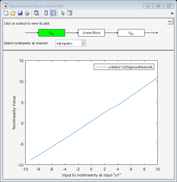
nlhwPlot(model1)

Explore the various plots in the plot window by clicking one of the three blocks that represent the model:

• uNL - Input nonlinearity, representing the static nonlinearity at the input ( model.InputNonlinearity ) to the Linear Block.

• Linear Block - Step, impulse,Bode and pole-zero plots of the embedded linear model ( model.LinearModel ). By default, a step plot is displayed.

• yNL - Output nonlinearity, representing the static nonlinearity at the output ( model.OutputNonlinearity ) of the Linear Block.

Specify Line Style for Multiple Hammerstein-Weiner Models

load iddata3
model1 = nlhw(z3,[4 2 1],idSigmoidNetwork(2),idGaussianProcess('Matern32'))

model1 =

Hammerstein-Wiener model with 1 output and 1 input

Linear transfer function corresponding to the orders nb = 4, nf = 2, nk = 1

Input nonlinearity: Sigmoid network with 2 units
Output nonlinearity: Gaussian process function using a Matern32 kernel
Sample time: 1 seconds

Status:                                       
Estimated using NLHW on time domain data "z3".
Fit to estimation data: 74.69%                
FPE: 1.732, MSE: 1.546

model2 = nlhw(z3, [4 2 1],[],'idSigmoidNetwork');
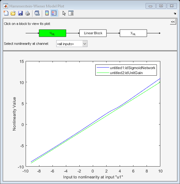
nlhwPlot(model1,'b-',model2,'g')

Specify Number of Samples, Time Samples, and Range of Input Nonlinearity

load iddata3
model1 = nlhw(z3,[4 2 1],idSigmoidNetwork(2),idGaussianProcess('Matern32'));
model2 = nlhw(z3, [4 2 1],[],'idSigmoidNetwork');
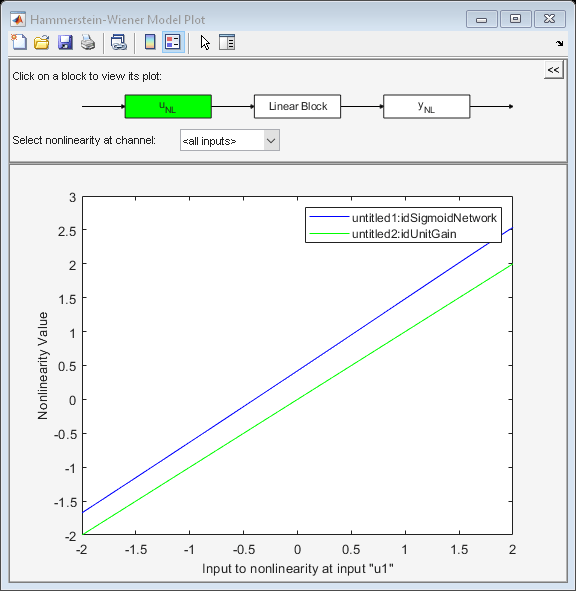
nlhwPlot(model1,'b-',model2,'g','NumberOfSamples',50,'time',10,'InputRange',[-2 2]);

Specify Time Samples, Frequency, and Range of Output Nonlinearity

load iddata3
model1 = nlhw(z3,[4 2 1],idSigmoidNetwork(2),idGaussianProcess('Matern32'));
model2 = nlhw(z3, [4 2 1],[],'idSigmoidNetwork');
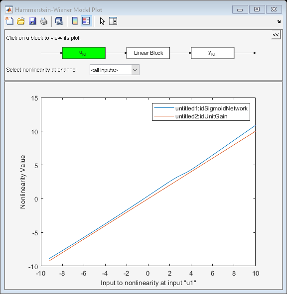
nlhwPlot(model1,model2,'time',1:500,'freq',{0.01,100},'OutputRange',[0 1000]);

Input Arguments

model — Estimated Hammerstein-Wiener model

idnlhw model

Estimated Hammerstein-Wiener model, specified as an idnlhw model object. Use nlhw to estimate the model.

LineSpec — Line style, marker symbol, and color

character vector

Line style, marker symbol, and color, specified as a character vector. LineSpec takes values such as 'b', 'b+:'. For more information, see the plot reference page in the MATLAB^® documentation.

Data Types: char

Name-Value Arguments

Specify optional pairs of arguments as Name1=Value1,...,NameN=ValueN, where Name is the argument name and Value is the corresponding value. Name-value arguments must appear after other arguments, but the order of the pairs does not matter.

Before R2021a, use commas to separate each name and value, and enclose Name in quotes.

Example: nlhwPlot(model,'NumberofSamples',10) specifies to use 10 data points for the input regressors.

NumberOfSamples — Number of data points to use for input regressors

100 (default) | positive integer

Number of data points to use for the input regressors when evaluating the nonlinearities at individual input or output channels, specified as a positive integer. This property does not affect the plots of the linear block.

Data Types: double

InputRange — Minimum and maximum regressor values for evaluating input nonlinearities

range of regressor values used during each model's estimation. (default) | positive integer | vector

Minimum and maximum regressor values to use when evaluating the nonlinearities at each input channel, specified as positive integers or [min max] vector, where minimum value is less than the maximum value.

You can use 'uRange' as a shortcut name for this property.

Data Types: double

OutputRange — Minimum and maximum regressor values for evaluating output nonlinearities

range of regressor values used during each model's estimation (default) | positive integer | vector

Minimum and maximum regressor values to use when evaluating the nonlinearities at each output channel, specified as positive integers or [min max] vector, where minimum value is less than the maximum value.

You can use 'yRange' as a shortcut name for this property.

Data Types: double

Time — Time samples to compute transient responses of the linear block

each model's dynamics determine the time samples used (default) | positive scalar | vector

The time samples at which the transient responses (step and impulse) of the linear block of the idnlhw model must be computed, specified as one of the following values:

• Positive scalar — Denotes end time for transient responses of all models. For example, 10.

• Vector of time instants — A double vector of uniformly sampled values denotes the time samples at which the transient response must be computed. For example, [0:0.1:10].

This property takes the same values as the step command on the model.

Frequency — Frequencies at which to compute the Bode response

automatically chosen inside the Nyquist frequency range (default) | [min max] range of positive scalars | vector of positive integers

Frequencies at which to compute the Bode response, specified as one of the following values:

• [Wmin Wmax] range — Frequency interval between Wmin and Wmax (in units rad/(model.TimeUnit)) covered using logarithmically placed points.

• Vector of non-negative frequency values — Allows computation of bode response at those frequencies.

By default, the response is computed at some automatically chosen frequencies inside the Nyquist frequency range. Frequencies above Nyquist frequency (pi/model.Ts) are ignored.

This property takes the same values as the bode command on the model.

More About

What is a Hammerstein-Wiener Plot?

A Hammerstein-Wiener plot displays the static input and output nonlinearities and linear responses of a Hammerstein-Wiener model.

Examining a Hammerstein-Wiener plot can help you determine whether you have selected a complicated nonlinearity for modeling your system. For example, suppose you use a piecewise-linear input nonlinearity to estimate your model, but the plot indicates saturation behavior. You can estimate a new model using the simpler saturation nonlinearity instead. For multivariable systems, you can use the Hammerstein-Wiener plot to determine whether to exclude nonlinearities for specific channels. If the nonlinearity for a specific input or output channel does not exhibit strong nonlinear behavior, you can estimate a new model after setting the nonlinearity at that channel to unit gain.

You can generate these plots in the System Identification app and at the command line. In the plot window, you can view the nonlinearities and linear responses by clicking one of the three blocks that represent the model:

• u_NL (input nonlinearity)— Click this block to view the static nonlinearity at the input to the Linear Block. The plot displays evaluate(M.InputNonlinearity,u) where M is the Hammerstein-Wiener model, and u is the input to the input nonlinearity block. For information about the blocks, see Structure of Hammerstein-Wiener Models.

• Linear Block — Click this block to view the Step, impulse, Bode, and pole-zero response plots of the embedded linear model (M.LinearModel). By default, a step plot of the linear model is displayed.

• y_NL (output nonlinearity) — Click this block to view the static nonlinearity at the output of the Linear Block. The plot displays evaluate(M.OutputNonlinearity,x), where x is the output of the linear block.

To learn more about how to configure the linear and nonlinear blocks plots, see Configuring a Hammerstein-Wiener Plot.

Version History

Introduced in R2023a

R2023a: nlhwPlot Replaces idnlhw/plot

nlhwPlot replaces the functionality of the idnlhw/plot method of idnlhw. Other than the function name, there are no functionality changes.

idnlhw/plot continues to work with idnlhw models. Use of idnlhw/plot is not recommended.