idnlarx/linearize
Linearize nonlinear ARX model
Syntax
SYS = linearize(NLSYS,U0,X0)
Description
SYS = linearize(NLSYS,U0,X0) linearizes
a nonlinear ARX model about the specified operating point U0 and X0.
The linearization is based on tangent linearization. For more information
about the definition of states for idnlarx models,
see Definition of idnlarx States.
Input Arguments
NLSYS:idnlarxmodel.U0: Matrix containing the constant input values for the model.X0: Model state values. The states of a nonlinear ARX model are defined by the time-delayed samples of input and output variables. For more information about the states of nonlinear ARX models, see thegetDelayInforeference page.
Note
To estimate U0 and X0 from operating point
specifications, use the idnlarx/findop command.
Output Arguments
SYSis anidssmodel.When the Control System Toolbox™ product is installed,
SYSis an LTI object.
Examples
Linearize a nonlinear ARX model around an operating point corresponding to a simulation snapshot at a specific time.
Load sample data.
load iddata2Estimate nonlinear ARX model from sample data.
nlsys = nlarx(z2,[4 3 10],idTreePartition,'custom',...
  {'sin(y1(t-2)*u1(t))+y1(t-2)*u1(t)+u1(t).*u1(t-13)',...
   'y1(t-5)*y1(t-5)*y1(t-1)'},'nlr',[1:5, 7 9]);
Plot the response of the model for a step input.
step(nlsys, 20)
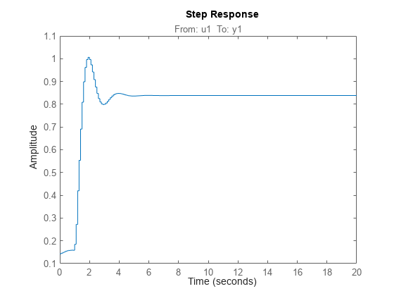
The step response is a steady-state value of 0.8383 at T = 20 seconds.
Compute the operating point corresponding to T = 20.
stepinput = iddata([],[zeros(10,1);ones(200,1)],nlsys.Ts);
[x,u] = findop(nlsys,'snapshot',20,stepinput);
Linearize the model about the operating point corresponding to the model snapshot at T = 20.
sys = linearize(nlsys,u,x);
Validate the linear model.
Apply a small perturbation delta_u to the steady-state input of the nonlinear model nlsys. If the linear approximation is accurate, the following should match:
The response of the nonlinear model
y_nlto an input that is the sum of the equilibrium level and the perturbationdelta_u.The sum of the response of the linear model to a perturbation input
delta_uand the output equilibrium level.
Generate a 200-sample perturbation step signal with amplitude 0.1.
delta_u = [zeros(10,1); 0.1*ones(190,1)];
For a nonlinear system with a steady-state input of 1 and a steady-state output of 0.8383, compute the steady-state response y_nl to the perturbed input u_nl. Use equilibrium state values x computed previously as initial conditions.
u_nl = 1 + delta_u;
y_nl = sim(nlsys,u_nl,x);
Compute response of linear model to perturbation input and add it to the output equilibrium level.
y_lin = 0.8383 + lsim(sys,delta_u);
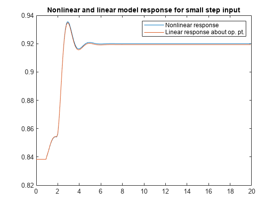
Compare the response of nonlinear and linear models.
time = (0:0.1:19.9)';
plot(time,y_nl,time,y_lin)
legend('Nonlinear response','Linear response about op. pt.')
title('Nonlinear and linear model response for small step input')
Algorithms
The following equations govern the dynamics of an idnlarx model:
where X(t) is a state vector, u(t) is the input, and y(t) is the output. A and B are constant matrices. is [y(t), u(t)]T.
The output at the operating point is given by
y* = f(X*, u*)
where X* and u* are the state vector and input at the operating point.
The linear approximation of the model response is as follows:
where
Note
For linear approximations over larger input ranges, use linapp.
Version History
Introduced in R2014b