ar

Estimate parameters when identifying AR model or ARI model for scalar time series

Syntax

sys = ar(y,n)

sys = ar(y,n,approach,window)

sys = ar(y,n,___,Name,Value)

sys = ar(y,n,___,opt)

[sys,refl] = ar(y,n,approach,___)

Description

sys = ar(y,n) estimates the parameters of an AR idpoly model sys of order n using a least-squares method. The model properties include covariances (parameter uncertainties) and estimation goodness of fit. y can be an output-only iddata object, a numeric vector, or a timetable.

sys = ar(y,n,approach,window) uses the algorithm specified by approach and the prewindowing and postwindowing specification in window. To specify window while accepting the default value for approach, use [] in the third position of the syntax.

sys = ar(y,n,___,Name,Value) specifies additional options using one or more name-value pair arguments. For instance, using the name-value pair argument 'IntegrateNoise',1 estimates an ARI model, which is useful for systems with nonstationary disturbances. Specify Name,Value after any of the input argument combinations in the previous syntaxes.

sys = ar(y,n,___,opt) specifies estimation options using the option set opt.

[sys,refl] = ar(y,n,approach,___) returns an AR model along with the reflection coefficients refl when approach is the lattice-based method 'burg' or 'gl'.

Examples

AR Model

Estimate an AR model and compare its response with the measured output.

Load the data, which contains the time series tt9 with noise.

load sdata9 tt9

Estimate a fourth-order AR model.

sys = ar(tt9,4)

sys =
Discrete-time AR model: A(z)y(t) = e(t)                            
  A(z) = 1 - 0.8369 z^-1 - 0.4744 z^-2 - 0.06621 z^-3 + 0.4857 z^-4
                                                                   
Sample time: 0.0039062 seconds
  
Parameterization:
   Polynomial orders:   na=4
   Number of free coefficients: 4
   Use "polydata", "getpvec", "getcov" for parameters and their uncertainties.

Status:                                                 
Estimated using AR ('fb/now') on time domain data "tt9".
Fit to estimation data: 79.38%                          
FPE: 0.5189, MSE: 0.5108                                
 

The output displays the polynomial containing the estimated parameters alongside other estimation details. Under Status, Fit to estimation data shows that the estimated model has 1-step-ahead prediction accuracy above 75%.

You can find additional information about the estimation results by exploring the estimation report, sys.Report. For instance, you can retrieve the parameter covariance.

covar = sys.Report.Parameters.FreeParCovariance

covar = 4×4

    0.0015   -0.0015   -0.0005    0.0007
   -0.0015    0.0027   -0.0008   -0.0004
   -0.0005   -0.0008    0.0028   -0.0015
    0.0007   -0.0004   -0.0015    0.0014

For more information on viewing the estimation report, see Estimation Report.

Compare Burg's Method with Forward-Backward Approach

Given a sinusoidal signal with noise, compare the spectral estimates of Burg's method with those found using the forward-backward approach.

Generate an output signal and convert it into an iddata object.

y = sin([1:300]') + 0.5*randn(300,1);
y = iddata(y);

Estimate fourth-order AR models using Burg's method and using the default forward-backward approach. Plot the model spectra together.

sys_b = ar(y,4,'burg');
sys_fb = ar(y,4);
spectrum(sys_b,sys_fb)
legend('Burg','Forward-Backward')

The two responses match closely throughout most of the frequency range.

ARI Model

Estimate an ARI model, which includes an integrator in the noise source.

Load the data, which contains the time series ymat9 with noise. Ts contains the sample time.

load sdata9 ymat9 Ts

Integrate the output signal.

y = cumsum(ymat9);

Estimate an AR model with 'IntegrateNoise' set to true. Use the least-squares method 'ls'.

sys = ar(y,4,'ls','Ts',Ts,'IntegrateNoise',true);

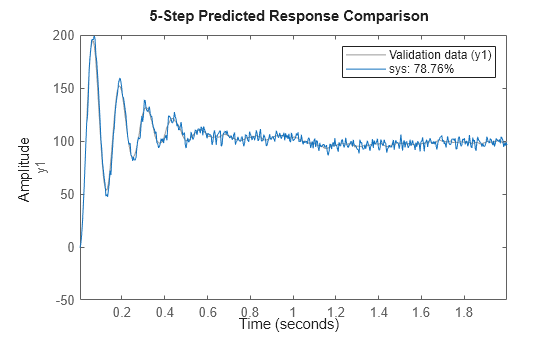
Predict the model output using 5-step prediction and compare the result with the integrated output signal y.

compare(y,sys,5)

Modify Default Options

Modify the default options for the AR function.

Load the data, which contains a time series z9 with noise.

load iddata9 z9

Modify the default options so that the function uses the 'ls' approach and does not estimate covariance.

opt = arOptions('Approach','ls','EstimateCovariance',false)

opt = 
Option set for the ar command:

              Approach: 'ls'
                Window: 'now'
            DataOffset: 0
    EstimateCovariance: 0
               MaxSize: 250000

Estimate a fourth-order AR model using the updated options.

sys = ar(z9,4,opt);

Retrieve Reflection Coefficients for Burg's Method

Retrieve reflection coefficients and loss functions when using Burg's method.

Lattice-based approaches such, as Burg's method 'burg' and geometric lattice 'gl', compute reflection coefficients and corresponding loss function values as part of the estimation process. Use a second output argument to retrieve these values.

Generate an output signal and convert it into an iddata object.

y = sin([1:300]') + 0.5*randn(300,1);
y = iddata(y);

Estimate a fourth-order AR model using Burg's method and include an output argument for the reflection coefficients.

[sys,refl] = ar(y,4,'burg');
refl

refl = 2×5

         0   -0.3562    0.4430    0.5528    0.2385
    0.8494    0.7416    0.5960    0.4139    0.3904

Input Arguments

y — Time-series data

iddata object | numeric vector | timetable

Time-series data, specified as one of the following:

• An iddata object that contains a single output channel and an empty input channel.

• A numeric column vector containing output-channel data. When you specify y as a vector, you must also specify the sample time Ts.

• A single-variable timetable.

For more information about working with estimation data types, see Data Domains and Data Types in System Identification Toolbox.

n — Model order

positive integer

Model order, specified as a positive integer. The value of n determines the number of A parameters in the AR model.

Example: ar(idy,2) computes a second-order AR model from the single-channel iddata object idy

approach — Algorithm for computing AR model

'fb' (default) | 'burg' | 'gl' | 'ls' | 'yw'

Algorithm for computing the AR model, specified as one of the following values:

• 'burg': Burg's lattice-based method. Solves the lattice filter equations using the harmonic mean of forward and backward squared prediction errors.

• 'fb': (Default) Forward-backward approach. Minimizes the sum of a least-squares criterion for a forward model, and the analogous criterion for a time-reversed model.

• 'gl': Geometric lattice approach. Similar to Burg's method, but uses the geometric mean instead of the harmonic mean during minimization.

• 'ls': Least-squares approach. Minimizes the standard sum of squared forward-prediction errors.

• 'yw': Yule-Walker approach. Solves the Yule-Walker equations, formed from sample covariances.

All of these algorithms are variants of the least-squares method. For more information, see Algorithms.

Example: ar(idy,2,'ls') computes an AR model using the least-squares approach

window — Prewindowing and postwindowing

'now' | 'pow' | 'ppw' | 'prw

Prewindowing and postwindowing outside the measured time interval (past and future values), specified as one of the following values:

• 'now': No windowing. This value is the default except when you set approach to 'yw'. Only measured data is used to form regression vectors. The summation in the criteria starts at the sample index equal to n+1.

• 'pow': Postwindowing. Missing end values are replaced with zeros and the summation is extended to time N+n (N is the number of observations).

• 'ppw': Prewindowing and postwindowing. The software uses this value whenever you select the Yule-Walker approach 'yw', regardless of your window specification.

• 'prw': Prewindowing. Missing past values are replaced with zeros so that the summation in the criteria can start at time equal to zero.

Example: ar(idy,2,'yw','ppw') computes an AR model using the Yule-Walker approach with prewindowing and postwindowing.

opt — Estimation options

arOptions option set

Estimation options for AR model identification, specified as an arOptions option set. opt specifies the following options:

• Estimation approach

• Data windowing technique

• Data offset

• Maximum number of elements in a segment of data

For more information, see arOptions. For an example, see Modify Default Options.

Name-Value Arguments

Specify optional pairs of arguments as Name1=Value1,...,NameN=ValueN, where Name is the argument name and Value is the corresponding value. Name-value arguments must appear after other arguments, but the order of the pairs does not matter.

Before R2021a, use commas to separate each name and value, and enclose Name in quotes.

Example: 'IntegrateNoise',true adds an integrator in the noise source

OutputName — Output signal names

" " (default) | character vector | string

Output channel names for timetable data, specified as a string or a character vector. By default, the software interprets the last variable in tt as the sole output channel. When you want to select a different timetable variable for the output channel, use 'OutputName' to identify it. For example, sys = ar(tt,__,'OutputName',"y3") selects the variable y3 as the output channel for the estimation.

Ts — Sample time

1 (default) | positive scalar

Sample time, specified as the comma-separated pair consisting of 'Ts' and the sample time in seconds. If y is a numeric vector, then you must specify 'Ts'.

Example: ar(y_signal,2,'Ts',0.08) computes a second-order AR model with sample time of 0.08 seconds

IntegrateNoise — Add integrator to noise channel

false (default) | logical vector

Noise-channel integration option for estimating ARI models, specified as the comma-separated pair consisting of 'IntegrateNoise' and a logical. Noise integration is useful in cases where the disturbance is nonstationary.

When using 'IntegrateNoise', you must also integrate the output-channel data. For an example, see ARI Model.

Output Arguments

sys — AR or ARI model

idpoly model object

AR or ARI model that fits the given estimation data, returned as a discrete-time idpoly model object. This model is created using the specified model orders, delays, and estimation options.

Information about the estimation results and options used is stored in the Report property of the model. Report has the following fields.

Report Field	Description
Status	Summary of the model status, which indicates whether the model was created by construction or obtained by estimation
Method	Estimation command used
Fit	Quantitative assessment of the estimation, returned as a structure. See Loss Function and Model Quality Metrics for more information on these quality metrics. The structure has these fields. FitPercent — Normalized root mean squared error (NRMSE) measure of how well the response of the model fits the estimation data, expressed as the percentage fitpercent = 100(1-NRMSE) LossFcn — Value of the loss function when the estimation completes MSE — Mean squared error (MSE) measure of how well the response of the model fits the estimation data FPE — Final prediction error for the model AIC — Raw Akaike Information Criteria (AIC) measure of model quality AICc — Small-sample-size corrected AIC nAIC — Normalized AIC BIC — Bayesian Information Criteria (BIC)
Parameters	Estimated values of model parameters
OptionsUsed	Option set used for estimation. If no custom options were configured, this is a set of default options. See arOptions for more information.
RandState	State of the random number stream at the start of estimation. Empty, [], if randomization was not used during estimation. For more information, see rng.
DataUsed	Attributes of the data used for estimation, returned as a structure with the following fields. Name — Name of the data set Type — Data type Length — Number of data samples Ts — Sample time InterSample — Input intersample behavior, returned as one of the following values: 'zoh' — A zero-order hold maintains a piecewise-constant input signal between samples. 'foh' — A first-order hold maintains a piecewise-linear input signal between samples. 'bl' — Band-limited behavior specifies that the continuous-time input signal has zero power above the Nyquist frequency. InputOffset — Offset removed from time-domain input data during estimation. For nonlinear models, it is []. OutputOffset — Offset removed from time-domain output data during estimation. For nonlinear models, it is [].

For more information on using Report, see Estimation Report.

refl — Reflection coefficients and loss functions

array

Reflection coefficients and loss functions, returned as a 2-by-2 array. For the two lattice-based approaches 'burg' and 'gl', refl stores the reflection coefficients in the first row and the corresponding loss function values in the second row. The first column of refl is the zeroth-order model, and the (2,1) element of refl is the norm of the time series itself. For an example, see Retrieve Reflection Coefficients for Burg's Method.

More About

AR (Autoregressive) Model

The AR model structure has no input, and is given by the following equation:

$$A(q)y(t)=e(t)$$

This model structure accommodates estimation for scalar time-series data, which have no input channel. The structure is a special case of the ARX structure.

ARI (Autoregressive Integrated) Model

The ARI model is an AR model with an integrator in the noise channel. The ARI model structure is given by the following equation:

$$A(q)y(t)=\frac{1}{1-q^{-1}}e(t)$$

Algorithms

AR and ARI model parameters are estimated using variants of the least-squares method. The following table summarizes the common names for methods with a specific combination of approach and window argument values.

Method	Approach and Windowing
Modified covariance method	(Default) Forward-backward approach with no windowing
Correlation method	Yule-Walker approach with prewindowing and postwindowing
Covariance method	Least squares approach with no windowing. arx uses this routine

References

[1] Marple, S. L., Jr. Chapter 8. Digital Spectral Analysis with Applications. Englewood Cliffs, NJ: Prentice Hall, 1987.

Version History

Introduced in R2006a

R2022b: Time-domain estimation data is accepted in the form of timetables and matrices

Most estimation, validation, analysis, and utility functions now accept time-domain input/output data in the form of a single timetable that contains both input and output data or a pair of matrices that contain the input and output data separately. These functions continue to accept iddata objects as a data source as well, for both time-domain and frequency-domain data.