HullWhite1F

Create Hull-White one-factor model

Description

The Hull-White one-factor model is specified using the zero curve, alpha, and sigma parameters.

Specifically, the HullWhite1F model is defined using the following equation:

$$dr=[\theta (t)-a(t)r]dt+\sigma (t)dW$$

where

dr is the change in the short-term interest rate over a small interval.

r is the short-term interest rate.

Θ(t) is a function of time determining the average direction in which r moves, chosen such that movements in r are consistent with today's zero coupon yield curve.

α is the mean reversion rate.

dt is a small change in time.

σ is the annual standard deviation of the short rate.

W is the Brownian motion.

Creation

Syntax

HW1F = HullWhite1F(ZeroCurve,Alpha,Sigma)

Description

HW1F = HullWhite1F(ZeroCurve,Alpha,Sigma) creates a HullWhite1F (HW1F) object using the required arguments to set the Properties.

Properties

ZeroCurve — Zero curve

IRDataCurve object | RateSpec

Zero curve, specified as an output from IRDataCurve or a RateSpec that is obtained from intenvset. This is the zero curve used to evolve the path of future interest rates.

Data Types: object | struct

Alpha — Mean reversion

numeric

Mean reversion, specified either as a scalar or function handle which takes time as input and returns a scalar mean reversion value.

Data Types: double

Sigma — Volatility

numeric

Volatility, specified either as a scalar or function handle which takes time as input and returns a scalar mean volatility.

Data Types: double

Object Functions

simTermStructs

Simulate term structures for Hull-White one-factor model

Examples

Create a Hull-White One-Factor Model Using an IRDataCurve

Create a Hull-White one-factor model using an IRDataCurve.

Settle = datetime(2007,12,15);
CurveTimes = [1:5 7 10 20]';
ZeroRates = [.01 .018 .024 .029 .033 .034 .035 .034]';
CurveDates = daysadd(Settle,360*CurveTimes,1);
 
irdc = IRDataCurve('Zero',Settle,CurveDates,ZeroRates);
    
alpha = .1;
sigma = .01;
 
HW1F = HullWhite1F(irdc,alpha,sigma)

HW1F = 
  HullWhite1F with properties:

    ZeroCurve: [1x1 IRDataCurve]
        Alpha: @(t,V)inAlpha
        Sigma: @(t,V)inSigma

Use the simTermStructs method with the HullWhite1F model to simulate term structures.

SimPaths = simTermStructs(HW1F, 10,'nTrials',100);

Create a Hull-White One-Factor Model Using a RateSpec

Create a Hull-White one-factor model using a RateSpec.

Settle = datetime(2007,12,15);
CurveTimes = [1:5 7 10 20]';
ZeroRates = [.01 .018 .024 .029 .033 .034 .035 .034]';
CurveDates = daysadd(Settle,360*CurveTimes,1);
 
RateSpec = intenvset('Rates',ZeroRates,'EndDates',CurveDates,'StartDate',Settle);

alpha = .1;
sigma = .01;
 
HW1F = HullWhite1F(RateSpec,alpha,sigma)

HW1F = 
  HullWhite1F with properties:

    ZeroCurve: [1x1 IRDataCurve]
        Alpha: @(t,V)inAlpha
        Sigma: @(t,V)inSigma

Use the simTermStructs method with the HullWhite1F model to simulate term structures.

SimPaths = simTermStructs(HW1F, 10,'nTrials',100);

Simulate the Price of a Bond Using a Hull-White One-Factor Model Until the Bond's Maturity

Define the zero curve data.

Settle = datetime(2016,4,4);
ZeroTimes = [3/12 6/12 1 5 7 10 20 30]';
ZeroRates = [0.033 0.034 0.035 0.040 0.042 0.044 0.048 0.0475]';
ZeroDates = datemnth(Settle,ZeroTimes*12);
RateSpec = intenvset('StartDates', Settle,'EndDates', ZeroDates, 'Rates', ZeroRates)

RateSpec = struct with fields:
           FinObj: 'RateSpec'
      Compounding: 2
             Disc: [8x1 double]
            Rates: [8x1 double]
         EndTimes: [8x1 double]
       StartTimes: [8x1 double]
         EndDates: [8x1 double]
       StartDates: 736424
    ValuationDate: 736424
            Basis: 0
     EndMonthRule: 1

Define the bond parameters.

Maturity = datemnth(Settle,12*5);
CouponRate = 0;

Define the Hull-White parameters.

alpha = .1;
sigma = .01;
HW1F = HullWhite1F(RateSpec,alpha,sigma)

HW1F = 
  HullWhite1F with properties:

    ZeroCurve: [1x1 IRDataCurve]
        Alpha: @(t,V)inAlpha
        Sigma: @(t,V)inSigma

Define the simulation parameters.

nTrials = 100;
nPeriods = 12*5;
deltaTime = 1/12;
SimZeroCurvePaths = simTermStructs(HW1F, nPeriods,'nTrials',nTrials,'deltaTime',deltaTime);
SimDates = datemnth(Settle,1:nPeriods);

Preallocate and initialize for the simulation.

SimBondPrice = zeros(nPeriods+1,nTrials);
SimBondPrice(1,:,:) = bondbyzero(RateSpec,CouponRate,Settle,Maturity);
SimBondPrice(end,:,:) = 100;

Compute the bond values for each simulation date and path, note that you can vectorize over the trial dimension.

for periodidx=1:nPeriods-1
    simRateSpec = intenvset('StartDate',SimDates(periodidx),'EndDates',...
        datemnth(SimDates(periodidx),ZeroTimes*12),'Rates',squeeze(SimZeroCurvePaths(periodidx+1,:,:)));
    SimBondPrice(periodidx+1,:) = bondbyzero(simRateSpec,CouponRate,SimDates(periodidx),Maturity);
end

plot([Settle SimDates],SimBondPrice)
ylabel('Bond Price')
xlabel('Simulation Dates')
title('Simulated Bond Price')

Simulate the Total Return of a Bond Portfolio Until Maturity

Define the zero curve data.

Settle = datetime(2016,4,4);
ZeroTimes = [3/12 6/12 1 5 7 10 20 30]';
ZeroRates = [-0.01 -0.009 -0.0075 -0.003 -0.002 -0.001 0.002 0.0075]';
ZeroDates = datemnth(Settle,ZeroTimes*12);
RateSpec = intenvset('StartDates', Settle,'EndDates', ZeroDates, 'Rates', ZeroRates)

RateSpec = struct with fields:
           FinObj: 'RateSpec'
      Compounding: 2
             Disc: [8x1 double]
            Rates: [8x1 double]
         EndTimes: [8x1 double]
       StartTimes: [8x1 double]
         EndDates: [8x1 double]
       StartDates: 736424
    ValuationDate: 736424
            Basis: 0
     EndMonthRule: 1

Define the bond parameters for the five bonds in the portfolio.

Maturity = datemnth(Settle,12*5);  % All bonds have the same maturity
CouponRate = [0.035;0.04;0.02;0.015;0.042];  % Different coupon rates for the bonds
nBonds = length(CouponRate);

Define the Hull-White parameters.

alpha = .1;
sigma = .01;
HW1F = HullWhite1F(RateSpec,alpha,sigma)

HW1F = 
  HullWhite1F with properties:

    ZeroCurve: [1x1 IRDataCurve]
        Alpha: @(t,V)inAlpha
        Sigma: @(t,V)inSigma

Define the simulation parameters.

nTrials = 1000;
nPeriods = 12*5;
deltaTime = 1/12;
SimZeroCurvePaths = simTermStructs(HW1F, nPeriods,'nTrials',nTrials,'deltaTime',deltaTime);
SimDates = datemnth(Settle,1:nPeriods);

Preallocate and initialize for the simulation.

SimBondPrice = zeros(nPeriods+1,nBonds,nTrials);
SimBondPrice(1,:,:) = repmat(bondbyzero(RateSpec,CouponRate,Settle,Maturity)',[1 1 nTrials]);
SimBondPrice(end,:,:) = 100;

[BondCF,BondCFDates,~,CFlowFlags] = cfamounts(CouponRate,Settle,Maturity);
BondCF(CFlowFlags == 4) = BondCF(CFlowFlags == 4) - 100;
SimBondCF = zeros(nPeriods+1,nBonds,nTrials);

Compute bond values for each simulation date and path. Note that you can vectorize over the trial dimension.

for periodidx=1:nPeriods
    if periodidx < nPeriods
        simRateSpec = intenvset('StartDate',SimDates(periodidx),'EndDates',...
            datemnth(SimDates(periodidx),ZeroTimes*12),'Rates',squeeze(SimZeroCurvePaths(periodidx+1,:,:)));
        SimBondPrice(periodidx+1,:,:) = bondbyzero(simRateSpec,CouponRate,SimDates(periodidx),Maturity);
    end
    
    simidx = SimDates(periodidx) == BondCFDates;
    SimCF = zeros(1,nBonds);
    SimCF(any(simidx,2)) = BondCF(simidx);
    ReinvestRate = 1 + SimZeroCurvePaths(periodidx+1,1,:);
    SimBondCF(periodidx+1,:,:) = bsxfun(@times,bsxfun(@plus,SimBondCF(periodidx,:,:),SimCF),ReinvestRate);
end

Compute the total return series.

TotalCF = SimBondPrice + SimBondCF;

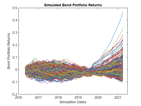
Assume the bond portfolio is equally weighted and plot the simulated bond portfolio returns.

TotalCF = squeeze(sum(TotalCF,2));

TotRetSeries = bsxfun(@rdivide,TotalCF(2:end,:),TotalCF(1,:)) - 1;
plot(SimDates,TotRetSeries)
ylabel('Bond Portfolio Returns')
xlabel('Simulation Dates')
title('Simulated Bond Portfolio Returns')

More About

Hull-White One-Factor Model

The Hull-White model is a single-factor, no-arbitrage yield curve model in which the short-term rate of interest is the random factor or state variable.

No-arbitrage means that the model parameters are consistent with the bond prices implied in the zero coupon yield curve.

References

[1] Brigo, D. and F. Mercurio. Interest Rate Models - Theory and Practice. Springer Finance, 2006.

[2] Hull, J. Options, Futures, and Other Derivatives. Prentice-Hall, 2011.

Version History

Introduced in R2013a