Time-Frequency Convolutional Network for EEG Data Classification

R2026b

This example shows how to classify electroencephalographic (EEG) time series from persons with and without epilepsy using a time-frequency convolutional network. The convolutional network predicts the class of the EEG data based on the continuous wavelet transform (CWT). The example compares the time-frequency network against a 1-D convolutional network. Unlike deep learning networks that use the magnitude or squared magnitude of the CWT (scalogram) as a preprocessing step, this example uses a differentiable scalogram layer. With a differentiable scalogram layer inside the network, you can put learnable operations before and after the scalogram. Layers of this type significantly expand the architectural variations that are possible with time-frequency transforms.

Data -- Description, Attribution, and Download Instructions

The data in this example were first analyzed and reported in:

Andrzejak, Ralph G., Klaus Lehnertz, Florian Mormann, Christoph Rieke, Peter David, and Christian E. Elger. “Indications of Nonlinear Deterministic and Finite-Dimensional Structures in Time Series of Brain Electrical Activity: Dependence on Recording Region and Brain State.” Physical Review E 64, no. 6 (2001). https://doi.org/10.1103/physreve.64.061907

The primary site for the data is Indications of nonlinear deterministic and finite-dimensional structures in time series of brain electrical activity: Dependence on recording region and brain state [dataset]

The data consists of five sets of 100 single-channel EEG recordings. The resulting single-channel EEG recordings were selected from 128-channel EEG recordings after visually inspecting each channel for obvious artifacts and satisfying a weak stationarity criterion. See the linked paper for details.

The original paper designates the class names for these five sets as A, B, C, D, and E. Each recording is 23.6 seconds in duration and sampled at a rate of 173.61 Hz. Each time series contains 4097 samples. The conditions are as follows:

A — Normal subjects with eyes open.

B — Normal subjects with eyes closed.

C — Seizure-free recordings from patients with epilepsy. Recordings obtained from hippocampus in the hemisphere opposite the epileptogenic zone.

D — Seizure-free recordings from patients with epilepsy. Recordings obtained from epileptogenic zone.

E — Recordings from patients with epilepsy showing seizure activity.

Download the EEG data set, EpilepsyEEGData.zip, file from the MathWorks® website, https://ssd.mathworks.com/supportfiles/WA/data/EpilepsyEEGData.zip. This example uses a copy of the data hosted in .mat file format. After downloading and unzipping, the data set folder contains a markdown file, LICENSE.md, with the required licensing information and attributions for the data. The LICENSE.md file additionally provides a link to the legal disclaimers associated with the original data. After unzipping the data, the EEGData folder contains subfolders Z, O, N, F, and S respectively. This table shows the correspondence between the labels Z, O, N, F, and S and those used in the original paper.

Original Paper	Data Set	Description
A	Z	Normal subjects with eyes open.
B	O	Normal subjects with eyes closed.
C	N	Seizure-free recordings from patients with epilepsy. Recordings obtained from hippocampus in the hemisphere opposite the epileptogenic zone.
D	F	Seizure-free recordings from patients with epilepsy. Recordings obtained from epileptogenic zone.
E	S	Recordings from patients with epilepsy showing seizure activity.

Each of these folders contain 100 .mat files. The datasetFolder is created under userpath. See the help for userpath if you wish to change this destination.

datasetZipFile = matlab.internal.examples.downloadSupportFile("WA","data/EpilepsyEEGData.zip");
datasetFolder = fullfile(fileparts(datasetZipFile),"EpilepsyEEGData");
if ~exist(datasetFolder,'dir')     
    unzip(datasetZipFile,datasetFolder);
end

Prepare Data for Training

The individual EEG time series are stored as .mat files in each of the Z, N, O, F, and S folders under dataDir. Use a signalDatastore to read the data. Create a categorical array of signal labels based on the file names.

sds = signalDatastore(fullfile(datasetFolder,"EEGData"),IncludeSubfolders=true,FileExtensions=".mat");
labels = filenames2labels(sds.Files,"ExtractBetween",[1 1]);

Read all the data. In a subsequent section, the signal labels are used to create subsets of the data.

eegData = readall(sds);

Given the five conditions present in the data, there are multiple meaningful and clinically informative ways to partition the data. One relevant way is to group the Z and O labels (non-epileptic subjects with eyes open and closed) as "Normal". Similarly, the two conditions recorded in epileptic subjects without overt seizure activity (F and N) may be grouped as "Pre-seizure". Finally, we designate the recordings obtained in epileptic subjects with seizure activity as "Seizure".

labels3Class = labels;
labels3Class = removecats(labels3Class,["F","N","O","S","Z"]);
labels3Class(labels == categorical("Z") | labels == categorical("O")) = ...
    categorical("Normal");
labels3Class(labels == categorical("F") | labels == categorical("N")) = ...
    categorical("Pre-seizure");
labels3Class(labels == categorical("S")) = categorical("Seizure");

Display the number of recordings in each of our derived categories. The summary shows three imbalanced classes with 100 recordings in the "Seizure" category and 200 recordings in each of the "Pre-seizure" and "Normal" categories.

summary(labels3Class)

labels3Class: 500×1 categorical

     Normal           200 
     Pre-seizure      200 
     Seizure          100 
     <undefined>        0 

Partition the data into a training set, a test set, and a validation set consisting of 70%, 20%, and 10% of the recordings, respectively.

idxSPN = splitlabels(labels3Class,[0.7 0.2 0.1]);
trainDataSPN = eegData(idxSPN{1});
trainLabelsSPN = labels3Class(idxSPN{1});
testDataSPN = eegData(idxSPN{2});
testLabelsSPN = labels3Class(idxSPN{2});
validationDataSPN = eegData(idxSPN{3});
validationLabelsSPN = labels3Class(idxSPN{3});

Examine the proportion of each condition across the three sets.

summary(trainLabelsSPN)

trainLabelsSPN: 350×1 categorical

     Normal           140 
     Pre-seizure      140 
     Seizure           70 
     <undefined>        0 

summary(validationLabelsSPN)

validationLabelsSPN: 50×1 categorical

     Normal           20 
     Pre-seizure      20 
     Seizure          10 
     <undefined>       0 

summary(testLabelsSPN)

testLabelsSPN: 100×1 categorical

     Normal           40 
     Pre-seizure      40 
     Seizure          20 
     <undefined>       0 

Because of the class imbalance, create weights proportional to the inverse class frequencies to use in training the deep learning model. This mitigates the tendency of the model to become biased toward more prevalent classes.

classwghts = numel(labels3Class)./(3*countcats(labels3Class));

Prior to training our time-frequency model, inspect the time series data and scalograms for the first example from each class. Use the helper function helperExamplePlot to plot representatives of each class.

helperExamplePlot(trainDataSPN,trainLabelsSPN)

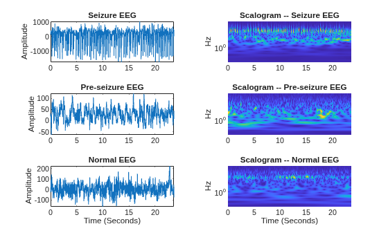
The scalogram is an ideal time-frequency transformation for time series data like EEG waveforms, which feature both slowly oscillating and transient phenomena.

Time-Frequency Deep Learning Network

Define a network that uses a time-frequency transformation of the input signal for classification.

netSPN = [
    sequenceInputLayer(1,MinLength=4097,Name="input",Normalization="zscore")
    convolution1dLayer(5,1,stride=2)
    cwtLayer(SignalLength=2047,IncludeLowpass=true,Wavelet="amor")
    maxPooling2dLayer([5,10])
    convolution2dLayer([5,10],5,Padding="same")
    maxPooling2dLayer([5,10])  
    batchNormalizationLayer
    reluLayer
    convolution2dLayer([5,10],10,Padding="same")
    maxPooling2dLayer([2,4])   
    batchNormalizationLayer
    reluLayer
    flattenLayer
    globalAveragePooling1dLayer
    dropoutLayer(0.4)
    fullyConnectedLayer(3)
    softmaxLayer
    ];

The network features an input layer, which normalizes the signals to have zero mean and unit standard deviation. Unlike [1], no preprocessing bandpass filter is used in this network. Rather, a learnable 1-D convolutional layer is used prior to obtaining the scalogram. We use a stride of 2 in the 1-D convolutional layer to downsample the size of the data along the time dimension. This reduces the computational complexity of the following scalogram. The next layer, cwtLayer (Wavelet Toolbox), obtains the scalogram (magnitude CWT) of the input signal. For each input signal, the output of the CWT layer is a sequence of time-frequency maps. This layer is configurable. In this case, we use the analytic Morlet wavelet and include the lowpass scaling coefficients. See [3] for another scalogram-based analysis of this data, and [2] for another wavelet-based analysis using the tunable Q-factor wavelet transform.

Subsequent to obtaining the scalogram, the network operates along both the time and frequency dimensions of the scalogram with 2-D operations until the flattenLayer. After flattenLayer, the model averages the output along the time dimension and uses a dropout layer to help prevent overfitting. The fully connected layer reduces the output along the channel dimension to equal the number of data classes (3).

We use the class weights previously computed to mitigate any network bias toward the underrepresented class. Create a custom loss function that takes predictions Y and targets T and returns the weighted cross-entropy loss.

lossFcn = @(Y,T)crossentropy(Y,T,classwghts,...
    NormalizationFactor="all-elements", ...
    WeightsFormat="C");

Specify the network training options. Output the network with the best validation loss.

options = trainingOptions("adam", ...
    MaxEpochs=40, ...
    MiniBatchSize=20, ...
    Shuffle="every-epoch",...
    Plots="training-progress",...
    ValidationData={validationDataSPN,validationLabelsSPN},...
    L2Regularization=1e-2,...
    OutputNetwork="best-validation-loss",...
    Verbose=false, ...
    Metrics="accuracy");

Train the neural network using the trainnet function. For weighted classification, use the custom cross-entropy function. By default, the trainnet function uses a GPU if one is available. Training on a GPU requires a Parallel Computing Toolbox™ license and a supported GPU device. For information on supported devices, see GPU Computing Requirements (Parallel Computing Toolbox). Otherwise, the trainnet function uses the CPU. To select the execution environment manually, use the ExecutionEnvironment training option.

trainedNetSPN = trainnet(trainDataSPN,trainLabelsSPN,netSPN,lossFcn,options);

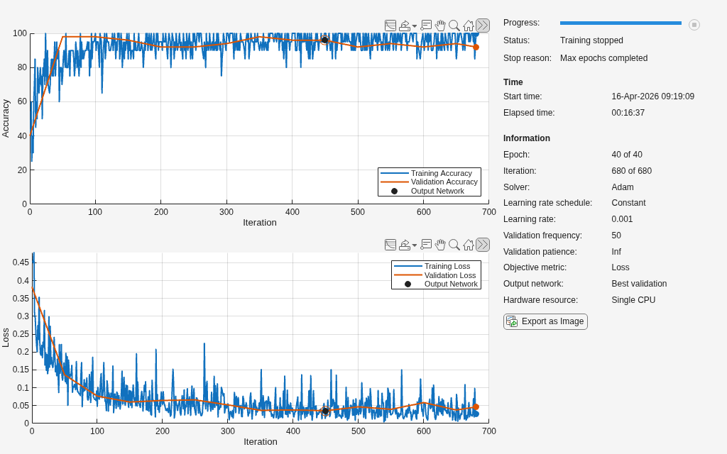
The training shows good agreement between the training and validation data sets.

After training completes, test the network on the held-out test set. Plot the confusion chart and examine the network's recall and precision.

scores = minibatchpredict(trainedNetSPN,testDataSPN);
classNames = unique(testLabelsSPN);
ypredSPN = scores2label(scores,classNames);
sum(ypredSPN == testLabelsSPN)/numel(testLabelsSPN)

ans = 
0.9700

hf = figure;
confusionchart(hf,testLabelsSPN,ypredSPN,RowSummary="row-normalized",ColumnSummary="column-normalized")

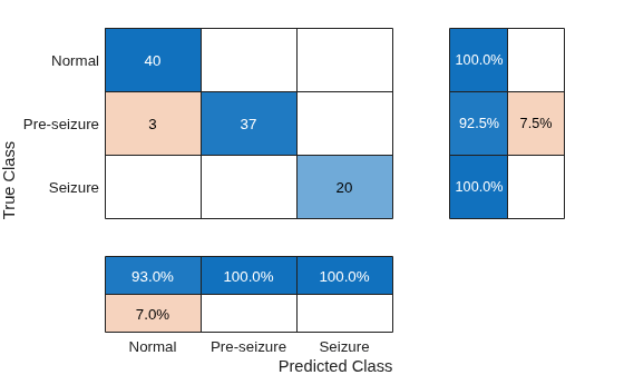
The confusion chart shows good performance on the test set. The row summaries in the confusion chart show the model's recall, while the column summaries show the precision. Both recall and precision generally fall between 93 and 100 percent. Performance was generally better for the "Seizure" and "Normal" classes than the "Pre-seizure" class.

1-D Convolutional Network

For reference, we compare the performance of the time-frequency deep learning network with a 1-D convolutional network which uses the raw time series as inputs. To the extent possible, the layers between the time-frequency network and time-domain network are kept equivalent. Note there are many variations of deep learning networks which can operate on the raw time series data. The inclusion of this particular network is presented as a point of reference and not intended as a rigorous comparison of time series network performance with that of the time-frequency network.

netconvSPN = [sequenceInputLayer(1,MinLength=4097,Name="input",Normalization="zscore")
    convolution1dLayer(5,1,stride=2)
    maxPooling1dLayer(10)
    batchNormalizationLayer
    reluLayer
    convolution1dLayer(5,5,Padding="same")
    batchNormalizationLayer
    reluLayer
    convolution1dLayer(5,10,Padding="same")
    maxPooling1dLayer(4)
    batchNormalizationLayer
    reluLayer
    globalAveragePooling1dLayer
    dropoutLayer(0.4)
    fullyConnectedLayer(3)
    softmaxLayer
    ];
trainedNetConvSPN = trainnet(trainDataSPN,trainLabelsSPN,netconvSPN,lossFcn,options);

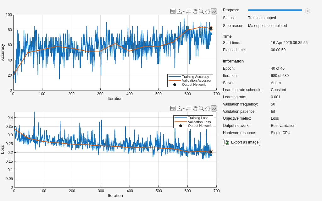
The training shows good agreement between accuracy on the training set and the validation set. However, the network accuracy during training is relatively poor. After training completes, test our model on the held-out test set. Plot the confusion chart and examine the model's recall and precision.

scores = minibatchpredict(trainedNetConvSPN,testDataSPN);
ypredconvSPN = scores2label(scores,classNames);
sum(ypredconvSPN == testLabelsSPN)/numel(testLabelsSPN)

ans = 
0.6900

hf = figure;
confusionchart(hf,testLabelsSPN,ypredconvSPN,RowSummary="row-normalized",ColumnSummary="column-normalized")

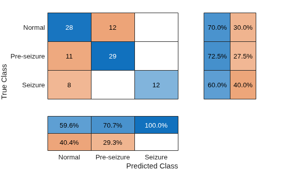
The recall and precision performance of the network is not surprisingly substantially less accurate than the time-frequency network.

Differentiating Pre-seizure vs Seizure

Another diagnostically useful partition of the data involves analyzing data only for the subjects with epilepsy and splitting the data into pre-seizure vs seizure data. As was done in the previous section, partition the data into training, test, and validation sets with 70%, 20%, and 10% splits of the data into Pre-seizure and Seizure examples. First, create the new labels in order to partition the data. Examine the number of examples in each class.

labelsPS = labels;
labelsPS = removecats(labelsPS,["F","N","O","S","Z"]);
labelsPS(labels == categorical("S")) = categorical("Seizure");
labelsPS(labels == categorical("F") | labels == categorical("N")) = categorical("Pre-seizure");
labelsPS(isundefined(labelsPS)) = [];
summary(labelsPS)

labelsPS: 300×1 categorical

     Seizure          100 
     Pre-seizure      200 
     <undefined>        0 

The resulting classes are unbalanced with twice as many signals in the "Pre-seizure" category as in the "Seizure" category. Partition the data and construct the class weights for the unbalanced classification.

idxPS = splitlabels(labelsPS,[0.7 0.2 0.1]);
trainDataPS = eegData(idxPS{1});
trainLabelsPS = labelsPS(idxPS{1});
testDataPS = eegData(idxPS{2});
testLabelsPS = labelsPS(idxPS{2});
validationDataPS = eegData(idxPS{3});
validationLabelsPS = labelsPS(idxPS{3});
classwghts = numel(labelsPS)./(2*countcats(labelsPS));

Use the same convolutional networks as in the previous analysis with modifications only in the fully connected layers by the differing number of classes.

netPS = [sequenceInputLayer(1,MinLength=4097,Name="input",Normalization="zscore")
    convolution1dLayer(5,1,"stride",2)
    cwtLayer(SignalLength=2047,IncludeLowpass=true,Wavelet="amor")
    averagePooling2dLayer([5,10])
    convolution2dLayer([5,10],5,Padding="same")
    maxPooling2dLayer([5,10])  
    batchNormalizationLayer
    reluLayer
    convolution2dLayer([5,10],10,Padding="same")
    maxPooling2dLayer([2,4])   
    batchNormalizationLayer
    reluLayer
    flattenLayer
    globalAveragePooling1dLayer
    dropoutLayer(0.4)
    fullyConnectedLayer(2)
    softmaxLayer
    ];

Train the network.

options = trainingOptions("adam", ...
    MaxEpochs=40, ...
    MiniBatchSize=32, ...
    Shuffle="every-epoch",...
    Plots="training-progress",...
    ValidationData={validationDataPS,validationLabelsPS},...
    L2Regularization=1e-2,...
    OutputNetwork="best-validation-loss",...
    Verbose=false, ...
    Metrics="accuracy");

lossFcn = @(Y,T)crossentropy(Y,T,classwghts,...
    NormalizationFactor="all-elements", ...
    WeightsFormat="C");

trainedNetPS = trainnet(trainDataPS,trainLabelsPS,netPS,lossFcn,options);

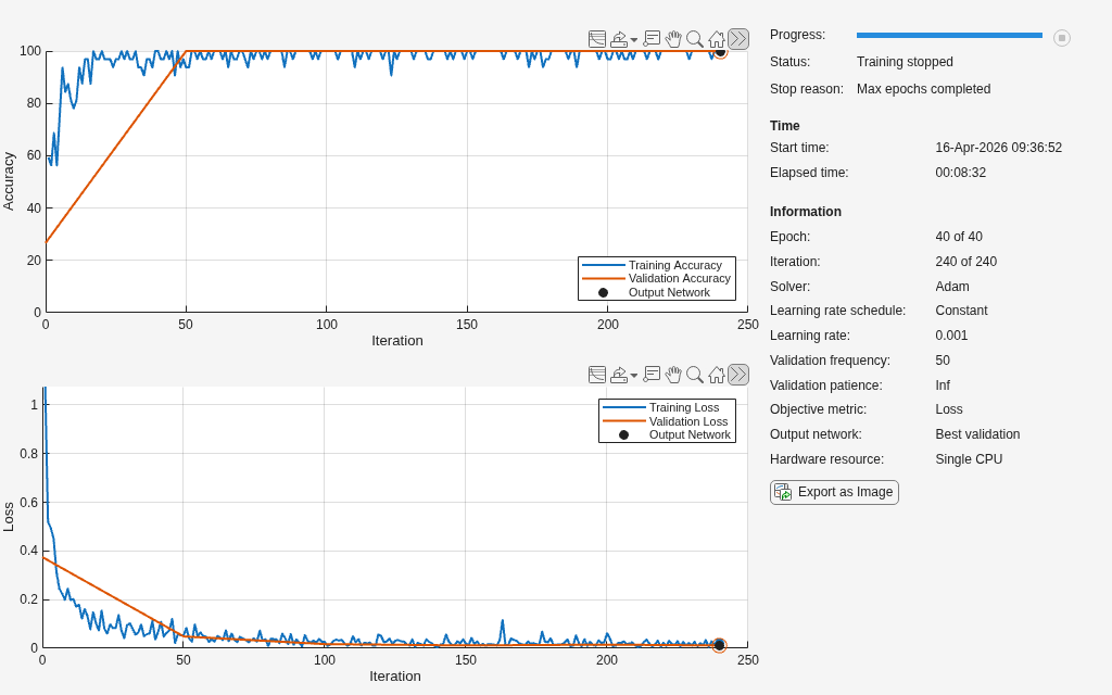
Examine the accuracy on the test set.

scores = minibatchpredict(trainedNetPS,testDataPS);
classNames = categories(trainLabelsPS);
ypredPS = scores2label(scores,classNames);
sum(ypredPS == testLabelsPS)/numel(testLabelsPS)

ans = 
0.9833

hf = figure;
confusionchart(hf,testLabelsPS,ypredPS,RowSummary="row-normalized",ColumnSummary="column-normalized")

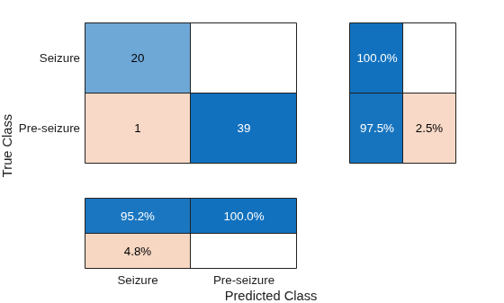
The time-frequency convolutional network shows excellent performance on the "Pre-seizure" vs "Seizure" data.

Summary

In this example, a time-frequency convolutional network was used to classify EEG recordings in persons with and without epilepsy. A crucial difference between this example and the scalogram network used in [3], was the use of a differentiable scalogram inside the deep learning model. This flexibility enables us to combine 1-D and 2-D deep learning layers in the same model, as well as place learnable operations before the time-frequency transform. The approach was compared against analogous 1-D convolutional networks. The 1-D convolutional networks were constructed to be as close to the time-frequency model as possible. It is likely that more optimal 1-D convolutional or recurrent networks can be designed for this data. As previously mentioned, the focus of the example was to construct a differentiable time-frequency network for real-world EEG data, not to conduct an in-depth comparison of the time-frequency model against competing time series models.

References

[1] Andrzejak, Ralph G., Klaus Lehnertz, Florian Mormann, Christoph Rieke, Peter David, and Christian E. Elger. “Indications of Nonlinear Deterministic and Finite-Dimensional Structures in Time Series of Brain Electrical Activity: Dependence on Recording Region and Brain State.” Physical Review E 64, no. 6 (2001). https://doi.org/10.1103/physreve.64.061907.

[2] Bhattacharyya, Abhijit, Ram Pachori, Abhay Upadhyay, and U. Acharya. “Tunable-Q Wavelet Transform Based Multiscale Entropy Measure for Automated Classification of Epileptic EEG Signals.” Applied Sciences 7, no. 4 (2017): 385. https://doi.org/10.3390/app7040385.

[3] Türk, Ömer, and Mehmet Siraç Özerdem. “Epilepsy Detection by Using Scalogram Based Convolutional Neural Network from EEG Signals.” Brain Sciences 9, no. 5 (2019): 115. https://doi.org/10.3390/brainsci9050115.

function helperExamplePlot(trainDataSPN,trainLabelsSPN)
% This function is for example use only. It may be changed or
% removed in a future release.
    szidx = find(trainLabelsSPN == categorical("Seizure"),1,"first");
    psidx = find(trainLabelsSPN == categorical("Pre-seizure"),1,"first");
    nidx = find(trainLabelsSPN == categorical("Normal"),1,"first");
    Fs = 173.61;
    t = 0:1/Fs:(4097*1/Fs)-1/Fs;
    [scSZ,f] = cwt(trainDataSPN{szidx},Fs,"amor");
    scSZ = abs(scSZ);
    scPS = abs(cwt(trainDataSPN{psidx},Fs,"amor"));
    scN = abs(cwt(trainDataSPN{nidx},Fs,"amor"));
    tiledlayout(3,2)
    nexttile
    plot(t,trainDataSPN{szidx}), axis tight
    title("Seizure EEG")
    ylabel("Amplitude")
    nexttile
    surf(t,f,scSZ), shading interp, view(0,90)
    set(gca,"Yscale","log"), axis tight
    title("Scalogram -- Seizure EEG")
    ylabel("Hz")
    nexttile
    plot(t,trainDataSPN{psidx}),axis tight
    title("Pre-seizure EEG")
    ylabel("Amplitude")
    nexttile
    surf(t,f,scPS), shading interp, view(0,90)
    set(gca,"Yscale","log"),axis tight
    title("Scalogram -- Pre-seizure EEG")
    ylabel("Hz")
    nexttile
    plot(t,trainDataSPN{nidx}), axis tight
    title("Normal EEG")
    ylabel("Amplitude")
    xlabel("Time (Seconds)")
    nexttile
    surf(t,f,scN), shading interp, view(0,90)
    set(gca,"Yscale","log"),axis tight
    title("Scalogram -- Normal EEG")
    ylabel("Hz")
    xlabel("Time (Seconds)")
end