Compress Sequence Classification Network for Road Damage Detection
This example shows how to compress a sequence classification network using pruning, projection, and quantization to meet a fixed memory requirement.
This example is step two in a series of examples that take you through training and compressing a neural network. You can run each step independently or work through the steps in order. The previous example shows how to train a neural network to classify timeseries of accelerometer data according to whether a vehicle drove over cracked or uncracked sections of pavement. Now, compress the network using Taylor pruning, projection, and quantization.
In this example, you choose an arbitrary split between pruning and projection to reach the required number of parameters before quantization. In the next example, you use Experiment Manager to determine what combination of pruning and projection results in the best accuracy while meeting the memory requirement.
Load Network and Data
Load the preprocessed data and trained network from step one of the series. If you have run the previous step, use the data and network in your workspace. Otherwise, the example prepares the data as described in Train Sequence Classification Network for Road Damage Detection and loads the saved network and training options. Add validation data to the training options.
if ~exist("XTrain","var") || ~exist("TTrain","var") || ...
        ~exist("XValidation","var") || ~exist("TValidation","var") || ...
        ~exist("XTest","var") || ~exist("TTest","var") || ...
        ~exist("netTrained","var") || ~exist("options","var") || ...
        ~exist("numClasses","var") || ~exist("classWeights","var") || ...
        ~exist("idxTrain","var") || ~exist("idxValidation","var") || ~exist("idxTest","var")
    load("RoadDamageAnalysisNetwork.mat")
    loadAndPreprocessDataForRoadDamageDetectionExample
end
options.ValidationData = {XValidation,TValidation};
Analyze and Test Network
Open the trained network in Deep Network Designer.
>> deepNetworkDesigner(netTrained)
Get a report on how much parameter reduction the network can achieve with each compression technique by clicking the Analyze for Compression button in the toolstrip.

The report shows that you can compress the network using pruning, projection, and quantization.
Test the accuracy of the trained network before compression using the testnet function.
accuracyTrained = testnet(netTrained,XTest,TTest,"accuracy")accuracyTrained = 97.0588
Set Compression Goals
Set the proportion of learnables to remove. The number you choose depends on your network and your memory requirements.
The size of the network in this example is 6.2 KB. To enable you to run this example quickly, the network and data set are small. The goal is to compress it to 0.5 KB.
Reducing the precision of the network parameters from single to 8-bit integer reduces the network memory by a factor of up to four. To reach a size of 0.5 KB, the network must first be compressed using pruning and projection to be smaller than 2 KB. To allow for some margin, aim to compress the network to smaller than 1.5 KB using pruning and projection.
Calculate the proportion of learnables to remove.
memoryUncompressed = 6.2;
memoryGoal = 1.5;
totalLearnablesReductionGoal = (memoryUncompressed - memoryGoal)/memoryUncompressed
totalLearnablesReductionGoal =
0.7581
Next, set the desired proportion of learnables to remove using only pruning. To perform only pruning and no projection, set pruningFraction to 1. To perform no pruning and only projection, set pruningFraction to 0.
In this example, aim to perform 50% pruning and 50% projection.
pruningFraction = 0.5;
It is not guaranteed that your network will meet these compression goals exactly.
In MATLAB®, Taylor pruning removes entire convolutional filters, instead of individual learnable parameters. So it is not always possible to meet the exact desired number of learnable parameters after pruning.
The maximum amount of pruning and projection can be insufficient to meet your goal. To check the maximum amount of compression using either pruning or projection, use Deep Network Designer. However, if you combine techniques, then you can compress the network further.
Projection compresses as much as possible without affecting neuron activation variance. If removing a greater proportion of learnables does not reduce the explained variance, then the
compressNetworkUsingProjectionfunction automatically removes a higher proportion of learnables. For example, if you specify a learnables reduction goal of0.2, and if the explained variance is the same for learnables reductions between0.2and0.5, then the function removes 50% of learnables.
Prune Network
The compressNetworkUsingTaylorPruning function prunes a network iteratively by repeating these steps:
Compute the importance score of each prunable filter.
Prune the least important filters.
Fine-tune the pruned network.
Calculate the target proportion of network learnable parameters to remove using Taylor pruning.
pruningLearnablesReductionGoal = totalLearnablesReductionGoal * pruningFraction;
Set the fine-tuning options. Use the same options that were used to train the original network, but use fewer training epochs.
optionsFineTuning = options;
optionsFineTuning.MaxEpochs = 10;
Compress the network using the compressNetworkUsingTaylorPruning function. To match the training configuration, specify the loss function as lossFcn. Specify the training options as optionsFineTuning. Specify the learnables reduction goal as pruningLearnablesReductionGoal. Remove approximately 2% of the original number of learnable parameters during each pruning iteration by specifying the learnables reduction increment as 0.02.
[netPruned,infoPruned] = compressNetworkUsingTaylorPruning(netTrained,XTrain,TTrain,lossFcn,optionsFineTuning, ...
    LearnablesReductionGoal = pruningLearnablesReductionGoal, ...
    LearnablesReductionIncrement = 0.02);
Compressed network has 38.4% fewer learnable parameters.
Pruning compressed 5 layers: "conv1d_1","batchnorm_1","conv1d_2","batchnorm_2","fc_1"
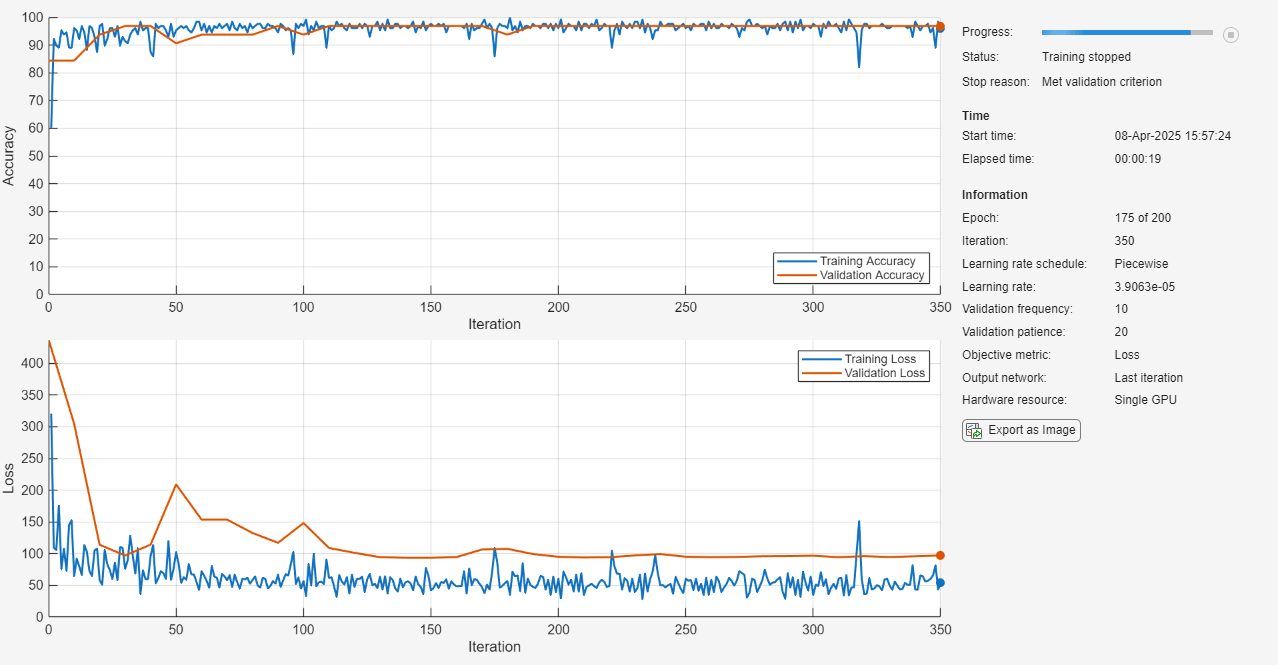
The pruning progress plot shows that in this example, the function performs 10 pruning iterations. During each iteration, the software tries to remove 2% of learnable parameters, until it exceeds the target learnables reduction. At the beginning of each pruning iteration, the loss spikes, but it recovers during fine-tuning.
Retrain Pruned Network
Retrain the pruned network using the trainnet function. Use the same loss function and training options used to train the network in the previous example.
netPruned = trainnet(XTrain,TTrain,netPruned,lossFcn,options);
Calculate the accuracy of the retrained model.
numLearnablesPruned = infoPruned.PruningHistory.NumLearnables(end);
accuracyPruned = testnet(netPruned,XTest,TTest,"accuracy")
accuracyPruned = 97.0588
Project Network
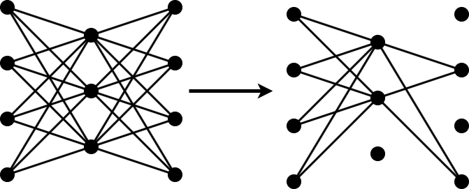
Projection allows you to convert large layers with many learnables to one or more smaller layers with fewer total learnable parameters.
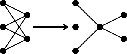
The compressNetworkUsingProjection function applies principal component analysis (PCA) to the training data to identify the subspace of learnables that result in the highest variance in neuron activations.
The total learnables reduction relates to the learnables reduction by pruning and projection in this way:
Calculate the proportion of parameters to remove using projection based on the proportion of learnables that were removed using pruning.
prunedLearnablesReduction = infoPruned.PruningHistory.LearnablesReduction(end);
projectionLearnablesReductionGoal = 1 - (1-totalLearnablesReductionGoal) / (1-prunedLearnablesReduction);
If you have not yet reached the overall compression goal, then project the network using the compressNetworkUsingProjection function.
if projectionLearnablesReductionGoal > 0
    [netProjected,infoProjection] = compressNetworkUsingProjection(netPruned,XTrain,LearnablesReductionGoal=projectionLearnablesReductionGoal);
end
Compressed network has 62.5% fewer learnable parameters.
Projection compressed 4 layers: "conv1d_1","conv1d_2","fc_1","fc_2"
Retrain Projected Network
If the network was projected, then retrain the network using the trainnet function. Use the same loss function and training options used to train the network in the previous example. If pruning removed enough learnable parameters to meet the parameters goal, then skip the projection and retraining steps. Calculate the remaining number of learnable parameters and the accuracy of the network.
if projectionLearnablesReductionGoal > 0
    options.MaxEpochs = 200;
    netProjected = trainnet(XTrain,TTrain,netProjected,lossFcn,options);
    numLearnablesProjected = countLearnables(netProjected)
    accuracyProjected = testnet(netProjected,XTest,TTest,"accuracy")
else
    netProjected = netPruned;
    numLearnablesProjected = numLearnablesPruned;
    accuracyProjected = accuracyPruned;
end
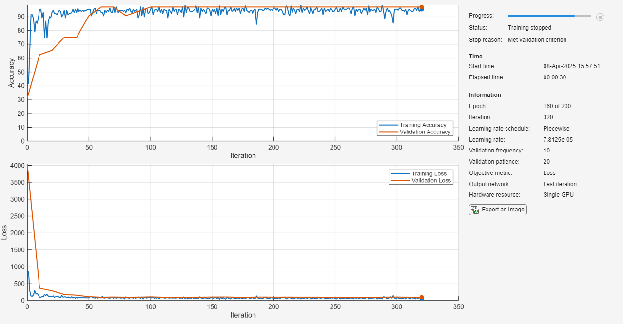
numLearnablesProjected =
352
accuracyProjected =
94.1176
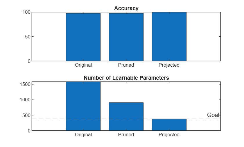
Compare the accuracy and number of learnables of the original, pruned, and projected networks.
numLearnablesTrained = countLearnables(netTrained);
numLearnablesGoal = (1 - totalLearnablesReductionGoal) * numLearnablesTrained;

figure
tiledlayout("vertical")
t1 = nexttile;
bar(t1,[accuracyTrained accuracyPruned accuracyProjected])
title(t1,"Accuracy")
xticklabels(["Original" "Pruned" "Projected"])

t2 = nexttile;
bar(t2,[numLearnablesTrained numLearnablesPruned numLearnablesProjected])
hold on
yline(numLearnablesGoal,'--','Goal')
hold off
title(t2,"Number of Learnable Parameters")
xticklabels(["Original" "Pruned" "Projected"])
Quantize Network
To see whether quantization can reduce the memory of the projected network enough to meet the memory goal of 0.5 KB, analyze the projected network for compression using Deep Network Designer.
>> deepNetworkDesigner(netProjected)
Get a report on how much parameter reduction the network can achieve with each compression technique by clicking the Analyze for Compression button in the toolstrip.
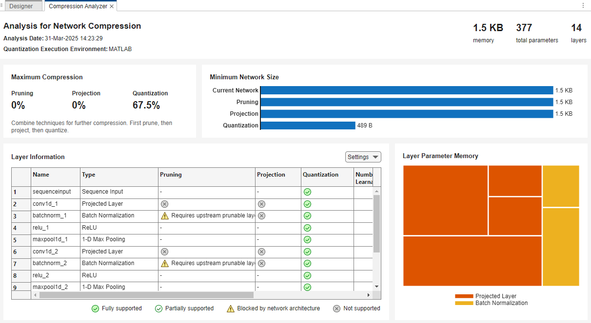
The report shows that quantization can reduce the memory of the network to below the memory goal of 0.5 KB. The report also indicates that you can not prune or project the network further. The presence of ProjectedLayer objects prevents the use of both techniques. To prune or project the network further, first unpack the projected layers using the unpackProjectedLayers function.
Next, to quantize the network, create a dlquantizer object from the fine-tuned projected network. Set the execution environment to MATLAB. When you use the MATLAB execution environment, the software uses the fi fixed-point data type to perform quantization. Using this data type requires a Fixed-Point Designer™ license.
quantObj = dlquantizer(netProjected,ExecutionEnvironment="MATLAB");Prepare your network for quantization using the prepareNetwork function. This function modifies the neural network to improve accuracy and avoid error conditions in the quantization workflow. In this example, the modifications include batch normalization layer fusion, equalization of layer parameters, and unpacking the projected layers.
prepareNetwork(quantObj)
Use the calibrate function to exercise the network with sample inputs and collect range information. The calibrate function exercises the network and collects the dynamic ranges of the weights and biases in the convolution and fully connected layers of the network and the dynamic ranges of the activations in all layers of the network.
calibrate(quantObj,XTrain);
Next, quantize the network using the quantize function. The function returns a quantized neural network object that enables visibility of the quantized layers, weights, and biases of the network, and the simulatable quantized inference behavior. To optimize the fit to the calibration data and improve the accuracy of the quantized network, set the exponent selection scheme to "histogram".
netQuantized = quantize(quantObj,ExponentScheme="histogram");Test the accuracy of the quantized network.
accuracyNetQuantized = testnet(netQuantized,XTest,TTest,"accuracy")accuracyNetQuantized = 91.1765
Test Results
Make predictions using the minibatchpredict function and convert the scores to labels using the onehotdecode function. By default, the minibatchpredict function uses a GPU if one is available.
YTest = minibatchpredict(netQuantized,XTest);
YTestLabels = onehotdecode(YTest,labels,1);
TTestLabels = onehotdecode(TTest,labels,1);
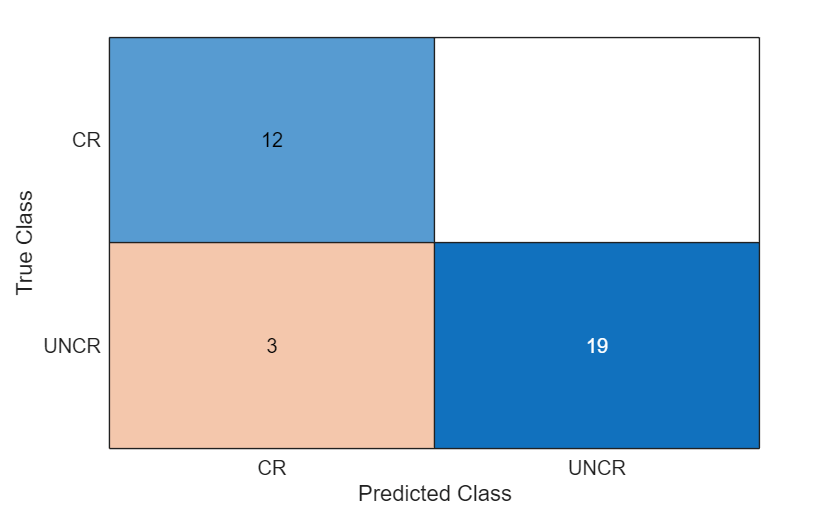
Display the classification results in a confusion chart.
figure
confusionchart(TTestLabels,YTestLabels)
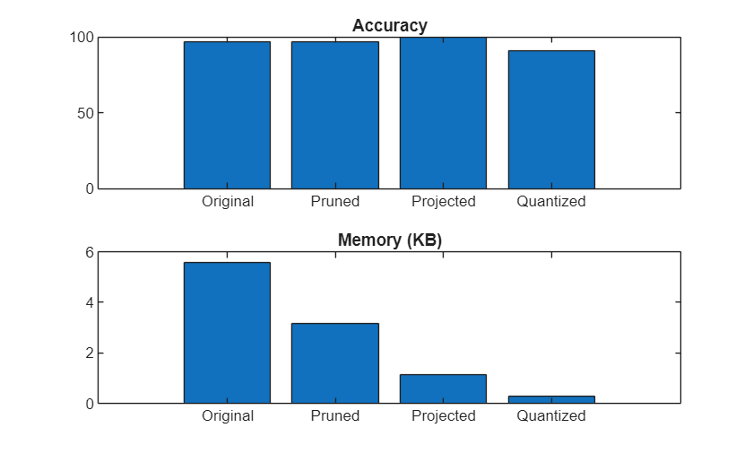
Compare the accuracy and memory after each compression step. The estimateLayerMemory function, defined at the bottom of this example, uses the estimateNetworkMetrics function to measure the memory of each supported layer. Not all layers in netTrained are supported, so the resulting number is less than the total network memory. For a list of supported layers, see estimateNetworkMetrics.
memoryNetTrained = estimateLayerMemory(netTrained);
memoryNetPruned = estimateLayerMemory(netPruned);
memoryNetProjected = estimateLayerMemory(unpackProjectedLayers(netProjected));
memoryNetQuantized = estimateLayerMemory(netQuantized);
memory = [memoryNetTrained memoryNetPruned memoryNetProjected memoryNetQuantized];
accuracy = [accuracyTrained accuracyPruned accuracyProjected accuracyNetQuantized];
Plot the accuracy and memory after each compression step.
figure
tiledlayout("vertical")
t1 = nexttile;
bar(t1,accuracy)
title(t1,"Accuracy")
xticklabels(["Original" "Pruned" "Projected" "Quantized"])

t2 = nexttile;
bar(t2,memory)
title(t2,"Memory (KB)")
xticklabels(["Original" "Pruned" "Projected" "Quantized"])
In the next step in the workflow, you use the code from this example to fine-tune the pruningFraction parameter to optimize the accuracy of the compressed network using Experiment Manager.
Next step: Tune Compression Parameters for Sequence Classification Network for Road Damage Detection. You can also open the next example using the openExample function.
>> openExample('deeplearning_shared/TuneCompressionParametersForRoadDamageDetectionNetworkExample')
Helper Functions
Calculate Memory of Supported Layers
function layerMemoryInKB = estimateLayerMemory(net)
    info = estimateNetworkMetrics(net);
    layerMemoryInMB = sum(info.("ParameterMemory (MB)"));
    layerMemoryInKB = layerMemoryInMB * 1000;
end
Count Number of Learnables
function numLearnables = countLearnables(net)
    numLearnables = sum(cellfun(@numel,net.Learnables.Value));
end
See Also
taylorPrunableNetwork | compressNetworkUsingProjection | dlquantizer | updatePrunables | updateScore | prepareNetwork | calibrate | quantize | trainnet | unpackProjectedLayers | minibatchpredict | onehotdecode | testnet