cscvn

“Natural” or periodic interpolating cubic spline curve

Syntax

curve = cscvn(points)

Description

curve = cscvn(points) returns a parametric variational, or natural, cubic spline curve (in ppform) passing through the given sequence points (:j), j = 1:end. The parameter value t(j) for the j-th point follows the Eugene Lee's [1] centripetal scheme, as accumulated square root of chord length:

$${\displaystyle \sum _{i<j}\sqrt{\Vert \text{points}(:,i+1)-\text{points }(:,i)\Vert {}_2}}$$

If the first and last point coincide and there are no other repeated points) then the function constructs a periodic cubic spline curve. However, double points result in corners.

Examples

Plot Interpolating Cubic Spline Curves

This example shows how to construct and plot several different interpolating cubic spline curves using the cscvn function.

This code generates a sequence of points and then plots the cubic spline generated from the cscvn function. The chosen points are marked as circles:

points=[0 1 1 0 -1 -1 0 0; 0 0 1 2 1 0 -1 -2]; 
fnplt(cscvn(points)); hold on, 
plot(points(1,:),points(2,:),'o'), hold off

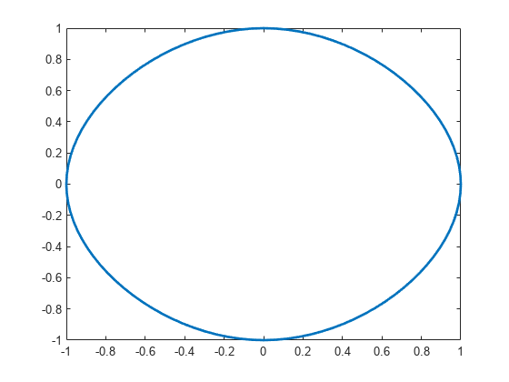
This code plots a circular curve through the four vertices of the standard diamond (because of the periodic boundary conditions enforced):

 fnplt(cscvn( [1 0 -1    0 1;0 1 0   -1 0] ))

This code shows a corner at the double point as well as at the curve endpoint:

 fnplt(cscvn( [1 0 -1 -1 0 1;0 1 0 0 -1 0] ))

Finally, this code generates a closed curve with one double point, which results in a corner. Dedicate this to your loved ones.

c=fnplt(cscvn([0 .82 .92 0 0 -.92 -.82 0; .66 .9 0 ...
-.83 -.83 0 .9 .66])); fill(c(1,:),c(2,:),'r'), axis equal

Input Arguments

points — Sequence of points

scalar | vector | matrix

Sequence of points at which the parametric "natural" cubic spline interpolates to, specified as a scalar, vector, or matrix.

Output Arguments

curve — Spline in ppform

spline structure

Spline in ppform, returned as a structure with these fields.

Form — Form of spline

pp

Form of the spline, returned as pp. pp indicates that the spline is given in piecewise polynomial form.

Breaks — Knot locations of spline

vector | cell array

Knot positions of the spline, returned as a vector or as a cell array of vectors for multivariate data. Vectors contain strictly increasing elements that represent the start and end of each of the intervals over which the polynomial pieces are defined.

Coefs — Coefficients of polynomials

matrix | array

Coefficients of polynomials for each piece, returned as a matrix or as an array for multivariate data.

Pieces — Number of polynomial pieces

scalar | vector

Number of polynomial pieces describing the spline, returned as a scalar or as a vector of numbers of pieces in each variable for multivariate data.

Order — Order of polynomials

scalar | vector

Order of the polynomial function describing each polynomial piece of the spline, returned as a scalar or as a vector containing the order in each variable for multivariate data.

Dim — Dimensionality

scalar

Dimensionality of the target function, returned as a scalar.

Algorithms

cscvn determines the break sequence t as

$$t_k=\{\begin{array}{l}0,k=1\\ {{\displaystyle \sum _{i=1}^{k-1}\left({\displaystyle \sum _{j=1}^d{(p_{i+1,j}-p_{i,j})}^2}\right)}}^{\frac{1}{4}},k>1\end{array}$$

where t_k is the element at position k in t, 1 ≤ k ≤ n–1, and p is the transpose of the d-by-n matrix points. If points contains repeated points, cscvn uses csape with periodic or variational end conditions to create the smooth pieces. cscvn returns the break sequence t in the breaks field of the curve output argument.

References

[1] E. T. Y. Lee. “Choosing nodes in parametric curve interpolation.” Computer-Aided Design 21 (1989), 363–370.

Version History

Introduced in R2006b