Control Design for Wind Turbine

This example discusses the control system for a 1.5 MW wind turbine. This example models the rotor dynamics as a simple first-order system, which neglects the flexible modes in the drivetrain, blades, and tower. The focus is on the design and validation of a gain-scheduled controller for the blade pitch in high-wind regime. For more details, see [1] and [2].

Turbine Model and Data

The rigid-body dynamics for the low-speed shaft are

$\mathit{J}\dot{\omega }={\mathit{T}}_{\mathit{a}}-{\mathit{T}}_{\mathit{g}}$,

where $\omega$ is the rotor speed, ${\mathit{T}}_{\mathit{a}}$ is the aerodynamic torque, and ${\mathit{T}}_{\mathit{g}}$ is the reaction torque from the generator connected to the high-speed shaft.

The aerodynamic torque depends on wind speed and blade pitch. Its calculation involves power coefficient data consisting of:

1. A grid TSRgrid of tip speed ratios (unitless). The tip speed ratio is $\mathrm{TSR}=\frac{\mathit{R}\omega }{\mathit{V}}$, where $\mathit{R}$ is the rotor radius (m), $\omega$ is the rotor speed (rad/s), and $\mathit{V}$ is the wind speed (m/s).

2. A grid Bgrid of blade pitch angles in degrees.

3. The table CpData of power coefficients ${\mathit{C}}_{\mathit{p}}$ (unitless) over the grid of tip speed ratios and pitch blade angles. The power generated by the turbine is $0.5{\rho \mathrm{AV}}^3{\mathit{C}}_{\mathit{p}}$, where $\rho$ is the air density (kg/m^3) and $\mathit{A}=\pi {\mathit{R}}^2$ is the rotor area (m).

This data is generated over a wide range of blade pitch and tip speed ratio values. The normal operating points correspond to ${\mathit{C}}_{\mathit{p}}>0$. Some entries of the table have ${\mathit{C}}_{\mathit{p}}<0$ (the turbine actually requires energy to operate at these points). Use points where ${\mathit{C}}_{\mathit{p}}<0$ with caution.

Load the data.

load WindCpData Bgrid TSRgrid CpData

This example uses the following values for the turbine physical parameters:

GBRatio = 88;      % Gearbox ratio, unitless
GBEff = 1.0;       % Gearbox efficiency, unitless (=1 for perfect eff.)
GenEff = 0.95;     % Generator efficiency, unitless (=1 for perfect eff.)
Jgen = 53;         % Generator Inertia about high-speed shaft, kg*m^2
Jrot = 3e6;        % Rotor inertia about low-speed shaft, kg*m^2
Jeq = Jrot+Jgen*GBRatio^2; % Equiv. inertia about low-speed shaft, kg*m^2
R = 35;            % Rotor radius, m
rho = 1.225;       % Air density, kg/m^3
wPA = 8.6;         % Pitch actuator natural frequency, rad/s
zetaPA = 0.8;      % Pitch actuator damping ratio, unitless
Bmax = 90;         % Maximum blade pitch angle, degrees
Kaw = 0.5;         % Anti-windup gain, rad/s/degree

The Simulink® model WindTurbineOpenLoop implements the simplified model of the rotor dynamics. Open the model.

open_system('WindTurbineOpenLoop')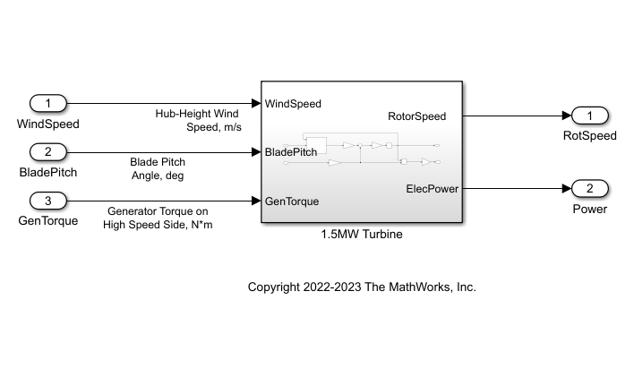

Rated Operating Point and Operating Regions

The power electronics on a wind turbine are sized to only produce a certain maximum power, called the rated power of the turbine (1.5 MW for this turbine). The rated torque, wind speed, and rotor speed correspond to the operating conditions where the turbine achieves the rated power.

Specify the rated power as 1.5 MW.

PRated = 1.5e6;

The rated rotor speed is 1800 rpm on high-speed shaft (HSS). Convert this speed to rad/s on the low-speed shaft (LSS).

wRatedHSS = 1800*(2*pi/60);
wRatedLSS = wRatedHSS/GBRatio;

The rated power is the product of the rated rotor speed, generator torque, and generator efficiency. Calculate the rate generator torque on the high speed shaft in N$\times$m.

GenTRated = PRated/(wRatedHSS*GenEff);

Specify the rated wind speed (m/s), which is the wind speed that achieves the rated rotor speed and rated generator torque. These values form an equilibrium point (when ${\mathit{C}}_{\mathit{p}}<{\mathit{C}}_{\mathit{p},\max }$).

WindRated = 11.2;

The controller switches between two operating regions delimited by the rated operating point:

• Region 2 (torque control): For wind speeds below rated, the blade pitch is set equal to its optimal (most efficient) value and the generator torque is set to a value proportional to ${\omega }^2$.

• Region 3 (blade pitch control): For wind speeds above rated, the generator torque is set to its rated value while the blade pitch is adjusted to maintain the rated rotor speed and deliver the rated power.

The generator torque in Region 2 is set to GenTRated = Kreg2$\times$wRatedLSS^2, where you choose $\mathrm{Kreg2}$ such that there is a smooth transition with Region 3. The rotor speed is wRatedLSS and generator torque is GenTRated.

Kreg2 = GenTRated / wRatedLSS^2

Kreg2 = 
1.8257e+03

Finally, compute the maximal power coefficient and corresponding optimal tip speed ratio and blade pitch angle.

CpMax = max(CpData,[],'all');
[i,j] = find(CpData==CpMax);
TSRopt = TSRgrid(i);
Bopt = Bgrid(j);

Optimal Operating Conditions as Function of Wind Speed

Compute the optimal steady-state operating conditions for wind speeds ranging from 4 to 24 m/s.

Specify the wind speed data for computing equilibrium points and initialize the arrays to store the rotor speeds on LSS, generator torques, blade pitch angles, and power delivered.

WindData = sort([4:0.5:24 WindRated]);

nW = numel(WindData);
wLSSeq = zeros(nW,1); 
GenTeq = zeros(nW,1); 
BladePitcheq = zeros(nW,1);
Peq = zeros(nW,1); 

In Region 2 (torque control), the rotor speed is proportional to the wind speed and the blade pitch is set to Bopt.

for i=1:nW
    Wind = WindData(i);
    if Wind<=WindRated
        % Region 2: Torque Control
        wLSSeq(i) = Wind/WindRated*wRatedLSS;
        GenTeq(i) = Kreg2*wLSSeq(i)^2;
        wHSS = wLSSeq(i)*GBRatio;
        Peq(i) = GenTeq(i)*wHSS*GenEff; % wRatedHSS*GenEff;
        BladePitcheq(i) = Bopt;
        % Populate operating point
        op(i) = operpoint('WindTurbineOpenLoop');
        op(i).States.x = wLSSeq(i);
        op(i).Inputs(1).u = Wind;
        op(i).Inputs(2).u = BladePitcheq(i);
        op(i).Inputs(3).u = GenTeq(i);
    end
end

In Region 3 (blade pitch control), the rotor speed and generator torque max out to their rated values wRatedLSS and GenTRated, respectively. Use findop to compute the blade pitch angle that maintains these steady-state values.

Specify trim options.

opt = findopOptions('DisplayReport','off', 'OptimizerType','lsqnonlin');
opt.OptimizationOptions.Algorithm = 'trust-region-reflective';

Perform batch trimming.

opspec = operspec('WindTurbineOpenLoop');
for i=1:nW
    Wind = WindData(i);
    if Wind>WindRated
        % Region 3: Blade Pitch Control
        wLSSeq(i) = wRatedLSS;
        GenTeq(i) = GenTRated;
        Peq(i) = PRated;
        % Trim condition
        opspec.States.Known = 1;
        opspec.States.SteadyState = 1;
        opspec.Inputs(1).Known=1;
        opspec.Inputs(1).u = Wind;
        opspec.Inputs(2).min = BladePitcheq(i-1);
        opspec.Inputs(3).Known=1;
        opspec.Inputs(3).u = GenTeq(i);
        % Compute corresponding operating point
        op(i) = findop('WindTurbineOpenLoop',opspec,opt);
        % Log steady-state blade pitch angle
        BladePitcheq(i) = op(i).Inputs(2).u;
    end
end

Plot the optimal settings of rotor speed, generator torque, electric power, and blade pitch angle as a function of wind speed. The red dot marks the rated operating point and transition between Regions 2 and 3.

clf
subplot(2,2,1)
plot(WindData,wLSSeq,'b',WindRated,wRatedLSS,'ro')
grid on
xlabel('Wind Speed, m/s')
title('Rotor Speed on LSS, rad/s')

subplot(2,2,2)
plot(WindData,GenTeq,'b',WindRated,GenTRated,'ro')
grid on
xlabel('Wind Speed, m/s')
title('Generator Torque on HSS, N*m')

subplot(2,2,3)
plot(WindData,Peq/1e6,'b',WindRated,PRated/1e6,'ro')
grid on
xlabel('Wind Speed, m/s')
title('Electric Power, MW')

subplot(2,2,4)
plot(WindData,BladePitcheq,'b')
grid on
xlabel('Wind Speed, m/s')
title('Blade Pitch, degrees')

Batch Linearization and LPV Model

Obtain a linearized model with offsets for the operating points from the previous section.

Specify linearization input and output points.

io = [linio('WindTurbineOpenLoop/WindSpeed',1,'in');
    linio('WindTurbineOpenLoop/BladePitch',1,'in');
    linio('WindTurbineOpenLoop/GenTorque',1,'in');
    linio('WindTurbineOpenLoop/1.5MW Turbine',1,'out'); % RotorSpeed
    linio('WindTurbineOpenLoop/1.5MW Turbine',2,'out')]; % Power

Linearize the model for each of the trim conditions. To store linearization offset information, use the info structure as an output argument.

linOpt = linearizeOptions('StoreOffsets',true);
[G,~,info] = linearize('WindTurbineOpenLoop',op,io,linOpt);
G.u = {'WindSpeed'; 'BladePitch'; 'GenTorque'};
G.y = {'RotorSpeed','Power'};
G.SamplingGrid = struct('WindSpeed',WindData);

Use ssInterpolant to construct an LPV model that interpolates these linearized models between grid points (wind speeds).

offsets = info.Offsets;
Glpv = ssInterpolant(G,offsets);

Linear Analysis for Fixed Wind Speeds

Split wind speeds into below rated (Region 2) and above rated (Region 3). Sample the LPV model of the turbine at these wind speeds.

[GR2,GR2offsets] = sample(Glpv,[],WindData( WindData<=WindRated ));
[GR3,GR3offsets] = sample(Glpv,[],WindData( WindData>=WindRated ));

Plot the Bode responses of linearization from blade pitch to rotor speed.

clf
bode(GR2(1,2,:),'b',GR3(1,2,:),'r-.')
legend('Region 2','Region 3','Location','Best')
grid on

Gain-Scheduled Blade Pitch Controller

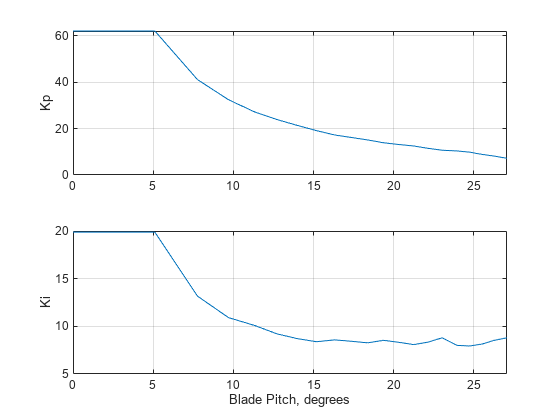
Design a gain-scheduled PI controller to adjust blade pitch in Region 3. The gains are scheduled on the blade pitch angle, which you can measure more reliably than wind speed. Recall that blade pitch must be adjusted to keep rotor speed, generator torque, and electric power from exceeding their rated values.

Sample the LPV plant for 20 values of wind speed between 11.5 and 24.

WindGS = linspace(11.5,24,20)';
BladePitchGS = interp1(WindData,BladePitcheq,WindGS);
GGS = sample(Glpv,[],WindGS);

For each wind speed, tune the PI gains to achieve a bandwidth of 0.66 rad/s.

wL = 0.66;      
opt = pidtuneOptions('PhaseMargin',70);
CPI = pidtune(-GGS(1,2),'pi',wL,opt);
Kp = CPI.Kp(:);
Ki = CPI.Ki(:);

Extend gain schedule to the entire range of blade pitch angles.

KpGS = [Kp(1); Kp; Kp(end)];
KiGS = [Ki(1); Ki; Ki(end)];
BladePitchGS = [0; BladePitchGS; Bmax];

Plot the gain schedules as a function of blade pitch angle.

clf
subplot(2,1,1)
plot(BladePitchGS,KpGS)
ylabel('Kp')
grid on
xlim(BladePitchGS([1 end-1]))
subplot(2,1,2)
plot(BladePitchGS,KiGS)
ylabel('Ki')
grid on
xlim(BladePitchGS([1 end-1]))
xlabel('Blade Pitch, degrees')

Nonlinear Closed-Loop Simulation

The Simulink model WindTurbineClosedLoop combines the turbine model, torque control for Region 2, and gain-scheduled blade pitch PI controller for Region 3.

open_system('WindTurbineClosedLoop')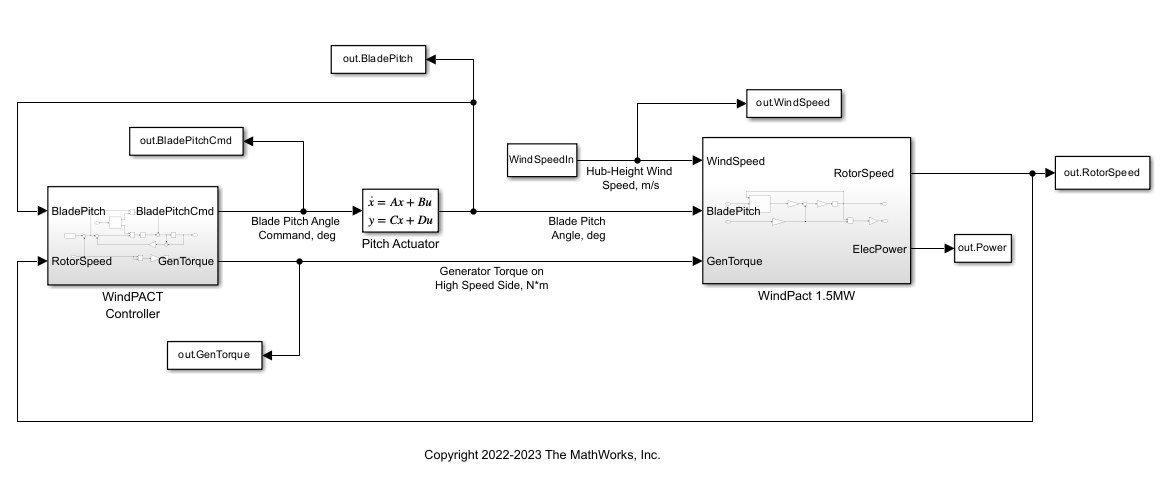

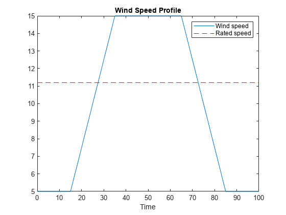
Use the following wind speed profile as input to the simulation.

V0 = 5;  
Vf = 15;
T1 = 15; 
T2 = 20;  
T3 = 30;   
Tf = 2*T1+2*T2+T3;
WindSpeedIn = [0 V0; T1 V0; T1+T2 Vf; T1+T2+T3 Vf; T1+2*T2+T3 V0; Tf V0];

t = (0:0.1:Tf)';
Wind = interp1(WindSpeedIn(:,1),WindSpeedIn(:,2),t);
clf
plot(t,Wind,[0 Tf],WindRated*[1 1],'r--')
xlabel('Time')
title('Wind Speed Profile')
legend('Wind speed','Rated speed')

Simulate the closed-loop response for this wind profile with proper initial conditions.

Specify the initial conditions for rotor speed, actuator state, and rotor speed error. This assumes V0 < WindRated, that is, Region 2.

w0 = V0/WindRated*wRatedLSS;
xPA0= [Bopt; 0]; 
e0 = wRatedLSS-w0;          

Specify the condition for controller integrator to be in steady-state:

0 = e0 + Kaw*(-KpGS(1)*e0-xK0-Bopt)

xK0 = e0*(1/Kaw-KpGS(1))-Bopt;

Simulate the model.

out = sim('WindTurbineClosedLoop',Tf);

Plot the power output.

Power = out.Power;
clf
plot(Power.Time,Power.Data/1e6)
ylabel('Power, MW')
grid on

Plot the other variables.

clf
subplot(2,2,1)
RotorSpeed = out.RotorSpeed;
plot(RotorSpeed.Time,RotorSpeed.Data,[0 Tf],wRatedLSS*[1 1],'r--')
title('Rotor Speed, rad/s') 
xlabel('Time, s')
grid on

subplot(2,2,2)
BladePitch = out.BladePitch;
plot(BladePitch.Time,BladePitch.Data);
title('Blade Pitch, degrees'); 
xlabel('Time, s')
grid on

subplot(2,2,3)
GenTorque = out.GenTorque;
plot(GenTorque.Time,GenTorque.Data,[0 Tf],GenTRated*[1 1],'r--')
title('Generator Torque, N*m')
xlabel('Time, s')
grid on;

subplot(2,2,4)
WindSpeed = out.WindSpeed;
plot(WindSpeed.Time,WindSpeed.Data,[0 Tf],WindRated*[1 1],'r--')
title('Wind Speed, m/s') 
xlabel('Time, s')
grid on

Closed-Loop LPV Simulation

From the LPV model Glpv of the turbine and the PI gain schedule, you can also construct a closed-loop LPV model and use it to validate the gain-scheduled controller in Region 3. First use ssInterpolant to create an LPV model of the gain-scheduled controller.

CPI = ss(0,permute(KiGS,[2 3 1]),1,permute(KpGS,[2 3 1]));
CPI.SamplingGrid = struct('BladePitch',BladePitchGS);

Clpv = ssInterpolant(CPI);
Clpv.InputName = 'RotSpeedErr';
Clpv.OutputName = 'BladePitchCmd';
Clpv.StateName = 'Controller';

The blade pitch actuator is modeled as a second-order system.

Actuator = ss([0 1; -wPA^2 -2*zetaPA*wPA],[0; wPA^2],[1 0],0);
Actuator.InputName = 'BladePitchCmd';
Actuator.OutputName = 'BladePitch';
Actuator.StateName = {'BladePitch','Act2'};

Use connect to build a closed-loop LPV model Tlpv including the LPV plant and the gain-scheduled PI controller. This closed-loop model depends on two parameters: wind speed and blade pitch angle.

SumBlk = sumblk('RotSpeedErr = RotorSpeed - RotSpeedCmd');

Tlpv = connect(Glpv,Clpv,Actuator,SumBlk,...
   {'WindSpeed','RotSpeedCmd','GenTorque'},...
   {'RotorSpeed','Power','BladePitch'});

Tlpv.ParameterName

ans = 2x1 cell
    {'WindSpeed' }
    {'BladePitch'}

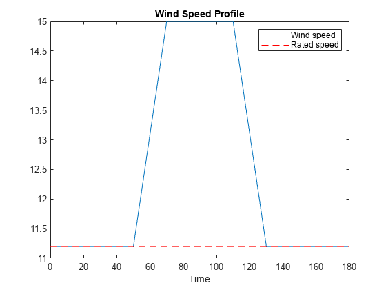
To validate the blade pitch controller, use a wind profile that lies entirely in Region 3.

V0 = WindRated;  
Vf = 15;
T1 = 50;  
T2 = 20;  
T3 = 40;  
Tf = 2*T1+2*T2+T3;
WindSpeedIn = [0 V0; T1 V0; T1+T2 Vf; T1+T2+T3 Vf; T1+2*T2+T3 V0; Tf V0];

t = (0:0.1:Tf)';
Wind = interp1(WindSpeedIn(:,1),WindSpeedIn(:,2),t);
clf 
plot(t,Wind,[0 Tf],WindRated*[1 1],'r--')
xlabel('Time') 
title('Wind Speed Profile')
legend('Wind speed','Rated speed')

Use lsim to simulate the closed-loop response. Define the parameter trajectory implicitly (wind speed is the first input and blade pitch angle is the first state of the actuator model).

% Inputs
u = zeros(numel(t),3);
u(:,1) = Wind;       % Wind profile
u(:,2) = wRatedLSS;  % Rotor speed
u(:,3) = GenTRated;  % Generator torque

% Initial condition
xinit = [wRatedLSS;Bopt;Bopt;0];

% Parameter trajectory
pFcn = @(t,x,u) [u(1);x(3)];  % x(3) = BladePitch

% LPV simulation
ylpv = lsim(Tlpv,u,t,xinit,pFcn);

Run the nonlinear simulation for the same wind profile.

w0 = wRatedLSS;  % Initial rotor speed, rad/s
xPA0 = [Bopt; 0];    % Initial actuator state
xK0 = -Bopt;        % integrator output
out = sim('WindTurbineClosedLoop',Tf);

Compare the LPV and nonlinear simulations.

RotorSpeed = out.RotorSpeed;
clf
subplot(3,1,1)
plot(RotorSpeed.Time,RotorSpeed.Data,t,ylpv(:,1),'--')
title('Rotor Speed, rad/s')
grid on
Power = out.Power;
subplot(3,1,2)
plot(Power.Time,Power.Data/1e6,t,ylpv(:,2)/1e6,'--')
title('Power, MW')
grid on
BladePitch = out.BladePitch;
subplot(3,1,3)
plot(BladePitch.Time,BladePitch.Data,t,ylpv(:,3),'--')
title('Blade Pitch, Degrees')
grid on
legend('Nonlinear','LPV','location','Best')

The LPV simulation accurately models rotor speed and blade pitch but underestimates the drop in power when wind speed decreases. This is because the LPV simulation fails to account for the drop in generator torque from the relationship GenTRated = Kreg2$\times$wRatedLSS^2.

Instead set u(:,3) = GenTRated, which fixes the generator torque to its rated value.

GenTorque = out.GenTorque;
clf
plot(GenTorque.Time,GenTorque.Data,[0 Tf],GenTRated*[1 1],'r--')
title('Generator Torque, N*m')
xlabel('Time, s')
grid on

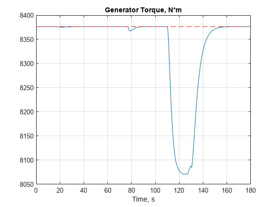
To improve accuracy, use the rotor speed data and previous relationship to estimate the generator torque data.

GenTorque = Kreg2 * ylpv(:,1).^2;
u(:,3) = min(GenTorque,GenTRated);
ylpv = lsim(Tlpv,u,t,xinit,pFcn);

Plot the responses.

clf
RotorSpeed = out.RotorSpeed;
subplot(3,1,1)
plot(RotorSpeed.Time,RotorSpeed.Data,t,ylpv(:,1),'--')
title('Rotor Speed, rad/s')
grid on
Power = out.Power;
subplot(3,1,2)
plot(Power.Time,Power.Data/1e6,t,ylpv(:,2)/1e6,'--')
title('Power, MW')
grid on
BladePitch = out.BladePitch;
subplot(3,1,3)
plot(BladePitch.Time,BladePitch.Data,t,ylpv(:,3),'--')
title('Blade Pitch, Degrees')
grid on
legend('Nonlinear','LPV','location','Best')

The LPV simulation now closely matches its nonlinear counterpart.

References

[1] Malcolm, D.J. and A.C. Hansen. “WindPACT Turbine Rotor Design Study: June 2000–June 2002 (Revised).” National Renewable Energy Laboratory, 2006 NREL/SR-500-32495. https://www.nrel.gov/docs/fy06osti/32495.pdf.

[2] Rinker, Jennifer and Dykes, Katherine. "WindPACT Reference Wind Turbines." National Renewable Energy Laboratory, 2018 NREL/TP-5000-67667. https://www.nrel.gov/docs/fy18osti/67667.pdf.