Main Content

SparseBalancedTruncation

Sparse balanced truncation model order reduction object

Since R2023b

    Description

    The SparseBalancedTruncation object stores model order reduction (MOR) specifications for the balanced truncation of sparse linear time-invariant (LTI) models.

    Creation

    The reducespec function creates a sparse balanced truncation model order reduction object when you use this syntax.

    R = reducespec(sys,"balanced")

    Here, sys is a sparse LTI model (sparss, mechss). The workflow uses this object to set up MOR tasks and store results. For the full model order reduction workflow, see Task-Based Model Order Reduction Workflow.

    Properties

    expand all

    This property is read-only.

    Hankel singular values, returned as a vector of size n-by-1. Here, n depends on the size of the rank of low-rank Gramian factors Lr and Lo. Additionally, nN, where N is the number of states of the original model.

    In state coordinates that equalize the input-to-state and state-to-output energy transfers, the Hankel singular values (HSVs) measure the contribution of each state to the input/output behavior. Hankel singular values relate to model order as singular values relate to matrix rank. In particular, small HSVs indicate states that you can discard to simplify the model.

    This property is read-only.

    Normalized state energies, returned as a vector of size n-by-1. Here, n depends on the size of the rank of low-rank Gramian factors Lr and Lo. Additionally, nN, where N is the number of states of the original model.

    These values measure the energy of each state relative to the state with maximum energy. The normalized state energy for the kth HSV is given by (σkσ1)2.

    This property is read-only.

    Bound on the absolute approximation error, returned as a vector of size n-by-1. Here, n depends on the size of the rank of low-rank Gramian factors Lr and Lo. Additionally, nN, where N is the number of states of the original model.

    This property is read-only.

    Low-rank Cholesky factor of the controllability Gramian, returned as a matrix.

    The controllability Gramian is approximately XrLrLrT.

    The computation of these low-rank approximations is based on [1] and [2].

    This property is read-only.

    Low-rank Cholesky factor of the observability Gramian, returned as a matrix.

    The observability Gramian is approximately XoLoLoT.

    The computation of these low-rank approximations is based on [1] and [2].

    This property is read-only.

    Relative residuals of Lyapunov equations, returned as a 1-by-2 vector. This property helps you tell if the algorithm has converged.

    Options for balanced truncation of LTI models, specified as a SparseBalancedTruncationOptions object. Use dot notation to configure options for R. For example R.Options.Focus = [10 1e5].

    For more information about available options, see SparseBalancedTruncationOptions.

    Object Functions

    processRun model order reduction algorithm
    view (balanced)Plot state contributions when using balanced truncation method
    getrom (balanced)Obtain reduced-order models when using balanced truncation method

    Examples

    collapse all

    This example shows how to perform balanced truncation of a sparse state-space model obtained from linearizing a thermal model of heat distribution in a circular cylindrical rod.

    Load the model data.

    load cylindricalRod.mat
    sys = sparss(A,B,C,D,E);
    size(sys)
    Sparse state-space model with 3 outputs, 1 inputs, and 7522 states.
    

    The thermal model contains 7522 states.

    Create a balanced truncation specification object for sys and run the algorithm.

    R = reducespec(sys,"balanced");
    R = process(R)
    Initializing...
    Running ADI with built-in shifts.........
    Running ADI with adaptive shifts..
    Solved Lyapunov equations to desired accuracy.
    
    R = 
      SparseBalancedTruncation with properties:
    
            Sigma: [40x1 double]
           Energy: [40x1 double]
            Error: [40x1 double]
               Lr: [7522x40 double]
               Lo: [7522x123 double]
        Residuals: [6.2579e-09 8.9726e-09]
          Options: [1x1 mor.SparseBalancedTruncationOptions]


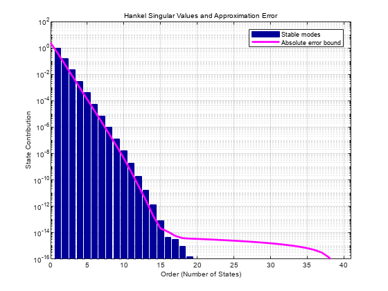
    Use the view command to visualize the state contributions as Hankel singular values

    view(R,"sigma")

    Obtain the reduced-order model with maximum error of 1e-6. This results in a model with order 8.

    rsys = getrom(R,MaxError=1e-6,Method="truncate");

    Compare the singular value response of the models.

    w = logspace(-7,-3,20);
    fsys = frd(sys,w);
    sigma(fsys,fsys-rsys,'r--')

    The reduced-order model is a good match for the full-order model.

    This example shows how to perform balanced truncation of an undamped second-order sparse model of a cantilever beam. Sparse balanced truncation is only supported for stable systems, but the algorithm allows you to implicitly add Rayleigh damping and enforce stability to perform model order reduction.

    Load the beam model.

    load linBeam.mat
    size(sys)
    Sparse second-order model with 1 outputs, 1 inputs, and 3303 degrees of freedom.
    

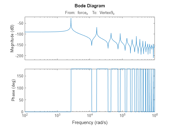
    Plot the Bode response.

    fsys = frd(sys,w);
    bode(fsys)

    The response shows that the model is undamped and has a dominant mode at 2639 rad/s.

    Create a model order reduction task.

    R = reducespec(sys,"balanced");

    Add the Rayleigh damping. Specify the natural frequency at 2700 rad/s near the dominant mode and the damping as 0.01.

    R.Options.Rayleigh = [2700,0.01];

    Analyze the model and compute the derived information.

    R = process(R);
    Initializing...
    Running ADI with built-in shifts........................................
    ..........................
    Running ADI with adaptive shifts...
    Solved Lyapunov equations to desired accuracy.
    

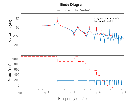
    Obtain a reduced-order model with order 20.

    rsys = getrom(R,Order=20,Method="truncate");
    bode(fsys,rsys,"r--",w)
    legend("Original sparse model","Reduced model")

    The reduced-order model is a good match for the sparse model.

    Algorithms

    The sparse balanced truncation algorithm performs these steps to reduce the input model G to the desired order k.

    1. Find the low-rank approximations Lr and Lo of the Gramian factors. This is based on the low-rank alternating directions implicit (LRADI) algorithm, which is an iterative method for solving the Lyapunov equations. For more details, see [1] and [2].

    2. Compute the HSVs σj based on the approximate controllability and observability Gramians.

    3. Obtain the reduced order model using the balanced model truncation with absolute error control [3] (see the Algorithms section of BalancedTruncation).

    References

    [1] Benner, Peter, Jing-Rebecca Li, and Thilo Penzl. “Numerical Solution of Large-Scale Lyapunov Equations, Riccati Equations, and Linear-Quadratic Optimal Control Problems.” Numerical Linear Algebra with Applications 15, no. 9 (November 2008): 755–77. https://doi.org/10.1002/nla.622.

    [2] Benner, Peter, Martin Köhler, and Jens Saak. “Matrix Equations, Sparse Solvers: M-M.E.S.S.-2.0.1—Philosophy, Features, and Application for (Parametric) Model Order Reduction.” In Model Reduction of Complex Dynamical Systems, edited by Peter Benner, Tobias Breiten, Heike Faßbender, Michael Hinze, Tatjana Stykel, and Ralf Zimmermann, 171:369–92. Cham: Springer International Publishing, 2021. https://doi.org/10.1007/978-3-030-72983-7_18.

    [3] Varga, A. “Balancing Free Square-Root Algorithm for Computing Singular Perturbation Approximations.” In [1991] Proceedings of the 30th IEEE Conference on Decision and Control, 1062–65. Brighton, UK: IEEE, 1991. https://doi.org/10.1109/CDC.1991.261486.
    Version History

    Introduced in R2023b