Main Content

BalancedTruncation

Balanced truncation model order reduction

Since R2023b

    Description

    The BalancedTruncation object stores model order reduction (MOR) specifications for the balanced truncation of ordinary (nonsparse) linear time-invariant (LTI) models.

    Creation

    The reducespec function creates a balanced truncation MOR object when you use this syntax.

    R = reducespec(sys,"balanced")

    Here, sys is any nonsparse LTI model. The workflow uses this object to set up MOR tasks and store results. For the full workflow, see Task-Based Model Order Reduction Workflow.

    Properties

    expand all

    This property is read-only.

    Hankel singular values σj,j=1N, returned as a vector of size N-by-1. Here, N is the number of states in the model.

    In state coordinates that equalize the input-to-state and state-to-output energy transfers, the Hankel singular values (HSVs) measure the contribution of each state to the input/output behavior. Hankel singular values relate to model order as singular values relate to matrix rank. In particular, small HSVs indicate states that you can discard to simplify the model.

    This property is read-only.

    Normalized state energy, returned as a vector of size N-by-1. Here, N is the number of states in the model.

    These values measure the energy of each state relative to the state with maximum energy. The normalized state energy for the kth HSV is given by (σkσ1)2.

    This property is read-only.

    Bound on absolute or relative approximation error, returned as a vector of size N-by-1. Here, N is the number of states in the model. For more information, see Algorithms.

    This property is read-only.

    Left-side matrix of transformation, returned as a matrix of size N-by-N. Here, N is the number of states in the model.

    The balanced truncation algorithm transforms the state-space realization (A, B, C) of a model to

    TLTATR=(A100A2),TLTB=(B1B2),CTR=(C1C2).

    The transformation scales the system and separates the stable and unstable parts. All modes of A1 are unstable and all modes of A2 are stable.

    This property is read-only.

    Right-side matrix of transformation, returned as a matrix of size N-by-N. Here, N is the number of states in the model.

    The algorithm transforms the state-space realization (A, B, C) of a model to

    TLTATR=(A100A2),TLTB=(B1B2),CTR=(C1C2).

    The transformation scales the system and separates the stable and unstable parts. All modes of A1 are unstable and all modes of A2 are stable.

    This property is read-only.

    Cholesky factor of the controllability Gramian of the stable part, returned as a matrix of size N-by-N. Here, N is the number of states in the model.

    The controllability Gramian of the stable part (A2, B2, C2) is Xr=LrLrT.

    This property is read-only.

    Cholesky factor of the observability Gramian of the stable part, returned as a matrix of size N-by-N. Here, N is the number of states in the model.

    The observability Gramian of the stable part (A2, B2, C2) is Xo=LoLoT.

    This property is read-only.

    Regularization level when R.Goal.Options is set to "relative", returned as a scalar value.

    Options for balanced truncation of LTI models, specified as a BalancedTruncationOptions object. Use dot notation to configure options for R. For example R.Options.Goal = "relative".

    For more information about available options, see BalancedTruncationOptions.

    Object Functions

    processRun model order reduction algorithm
    view (balanced)Plot state contributions when using balanced truncation method
    getrom (balanced)Obtain reduced-order models when using balanced truncation method

    Examples

    collapse all

    This example shows how to obtain a reduced-order model for a linear time-invariant (LTI) model using the balanced truncation method. In this example, you reduce a high-order model with a focus on the dynamics in a particular frequency range.

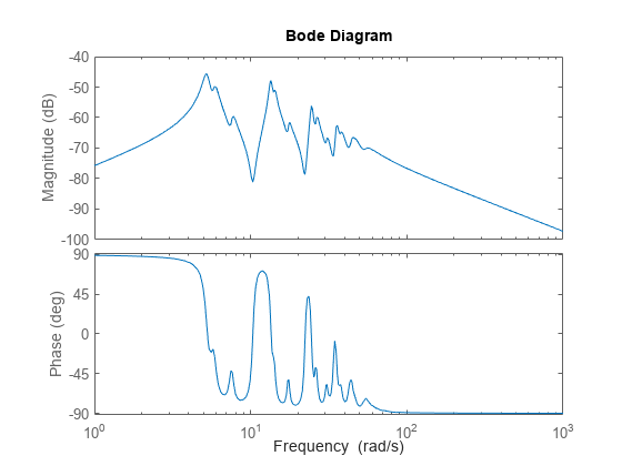
    Load a model and examine its frequency response.

    load('highOrderModel.mat','G')
    bodeplot(G)

    G is a 48th-order model with several large peak regions around 5.2 rad/s, 13.5 rad/s, and 24.5 rad/s, and smaller peaks scattered across many frequencies. Suppose that for your application you are only interested in the dynamics near the second large peak, between 10 rad/s and 22 rad/s. Focus the model reduction on the region of interest to obtain a good match with a low-order approximation.

    Create a model order reduction task and specify the desired frequency interval.

    R = reducespec(G,"balanced");
    R.Options.FreqIntervals = [10,22];

    Analyze the model and compute the derived information.

    R = process(R);

    Use the getrom function to retain all the modes between 10 rad/s and 22 rad/s.

    [rsys,info] = getrom(R,Order=[10,18],Method="truncate");

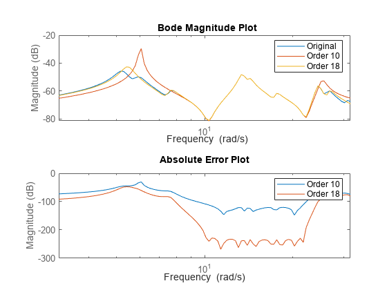
    Examine the frequency responses of the reduced-order models. Also, examine the difference between those responses and the original response (the absolute error).

    subplot(2,1,1);
    bodemag(G,rsys(:,:,1,1),rsys(:,:,2,1),logspace(0.5,1.5,100))
    title('Bode Magnitude Plot')
    legend("Original","Order 10", "Order 18")
    subplot(2,1,2);
    bodemag(G-rsys(:,:,1,1),G-rsys(:,:,2,1),logspace(0.5,1.5,100));
    title('Absolute Error Plot')
    legend('Order 10','Order 18');

    With the frequency-limited energy computation, even the 10th-order approximation is quite good in the region of interest.

    This example shows how to create a model order reduction specification for a dense LTI model using the balanced truncation method.

    For this example, generate a random discrete-time state-space model with 40 states.

    rng(0)
    sys = drss(40);

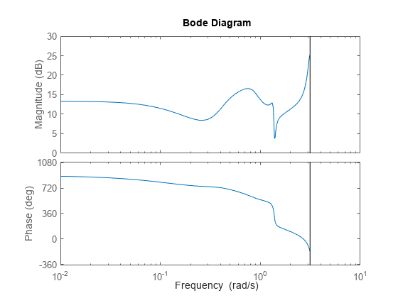
    Plot the Bode response.

    bode(sys)

    Create the specification object.

    R = reducespec(sys,"balanced");

    Notice that reducespec does not perform any computation and creates only the object. This allows you to set additional options before running the model order reduction algorithm, such as relative error control as the algorithm objective.

    R.Options.Goal = "relative";

    For balanced truncation, you can visualize the contributions in terms of the Hankel singular values or normalized energies. By default, the view function plots Hankel singular values.

    view(R)

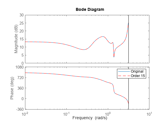
    For this example, select an order of 15 since it is the first order with a relative error less than 1e-4. In general, you select the order based on the desired absolute or relative fidelity. Then, compute the reduced-order model.

    rsys = getrom(R,Order=15);

    Plot the Bode response of both models.

    bode(sys,rsys,'r--')
    legend("Original","Order 15")

    This example shows how to improve the balanced truncation approximation with the help of frequency weights to emphasize accuracy in a particular frequency band.

    For this example, generate a random state-space model with 30 states, two outputs, and three inputs.

    rng(2)
    sys = rss(30,2,3);
    size(sys)
    State-space model with 2 outputs, 3 inputs, and 30 states.
    

    Create a model order reduction task.

    R = reducespec(sys,"balanced");

    Obtain the reduced order model.

    rsys = getrom(R,Order=19);
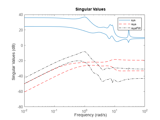
    sigma(sys,sys-rsys,"r--")
    legend("sys","sys-rsys")

    This reduced-order model does not provide a great approximation in the high frequencies. To improve the response, you can use the options to specify frequency weights to emphasize accuracy in a particular frequency band. These weights should have high gain in frequency bands of interest and low gain elsewhere.

    Specify the frequency weights with a high gain in the 3 rad/s to 100 rad/s band.

    wi = tf([1 0 0 0],[1 6 18 27])*eye(3);
    wo = tf(1,[0.01 1])*eye(2);
    R.Options.InputWeight = wi;
    R.Options.OutputWeight = wo;

    Obtain the reduced-order model.

    rsysFW = getrom(R,Order=19);
    sigma(sys,sys-rsys,"r--",sys-rsysFW,"k-.")
    legend({"sys","rsys","rsysFW"},FontSize=8)

    The model with frequency weighted reduction provides a better approximation across the higher frequencies.

    This example shows how you can use input and output scaling to emphasize accuracy of model order reduction in a particular channel of a MIMO model.

    Load the CD player state-space model.

    load cdromData.mat cdrom
    size(cdrom)
    State-space model with 2 outputs, 2 inputs, and 120 states.
    

    Create a model order reduction task.

    R = reducespec(cdrom,"balanced");

    Specify the input and output weights as static values such that the (1,2) channel is dominant.

    R.Options.InputWeight = diag([1e-3 1]); 
    R.Options.OutputWeight=diag([1 0.1]);

    Obtain the reduced-order model.

    rsys = getrom(R,MaxError=1e-2,Method="truncate");
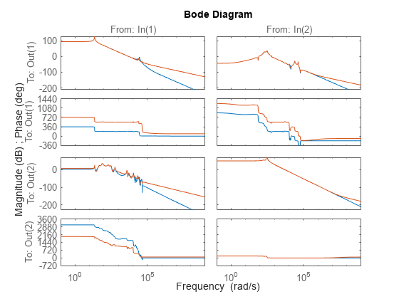
    bode(cdrom,rsys)

    The reduced-order model provides a good match for the scaled I/O channel.

    Model order reduction method controls the overall error of the MIMO model, so it is unlikely you get high relative accuracy on all channels when the gains are very different. Scaling an I/O channel helps you control the accuracy for that particular channel.

    Algorithms

    Balanced truncation first decomposes the system G into its stable and unstable parts:

    G=Gs+Gu

    When you specify R.Options.Goal as "absolute", the software uses the balanced truncation method of [1] to reduce Gs. This computes the HSVs σj based on the controllability and observability Gramians. For order r, the absolute error GsGr is bounded by 2j=r+1nσj. Here, n is the number of states in Gs.

    When you specify R.Options.Goal as "relative", the software uses the balanced stochastic truncation method of [2] to reduce Gs. For square Gs, this computes the HSVs σj of the phase matrix F=(W')1G, where W(s) is a stable, minimum-phase spectral factor of GG’:

    W'(s)W(s)=G(s)G'(s)

    For order r, the relative error Gs1(GsGr) is bounded by

    j=r+1H(1+σj1σj)12j=r+1nσj

    where 2j=r+1nσj1.

    References

    [1] Varga, A., "Balancing-Free Square-Root Algorithm for Computing Singular Perturbation Approximations," Proc. of 30th IEEE CDC, Brighton, UK (1991), pp. 1062-1065.

    [2] Green, M., "A Relative Error Bound for Balanced Stochastic Truncation", IEEE Transactions on Automatic Control, Vol. 33, No. 10, 1988
    Version History

    Introduced in R2023b