Main Content

view

Plot state contributions when using balanced truncation method

Since R2023b

    Description

    Use view to graphically analyze the model and select a model order reduction criteria from a model order reduction task created using reducespec. For BalancedTruncation and SparseBalancedTruncation objects, you can visualize the state contributions as either Hankel singular values or normalized state energies. For the full workflow, see Task-Based Model Order Reduction Workflow.

    view(R,type) creates a plot that helps you select the order of the reduced model. R specifies the model order reduction (MOR) specification object. Use the type argument to specify the plot type as either "sigma" or "energy".

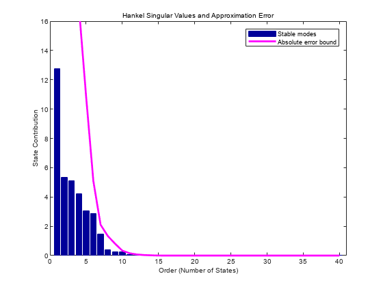
    view(R) plots the default plot type for the model order reduction algorithm of R. For balanced truncation methods, this syntax plots Hankel singular values and associated error bounds.

    view(___,Axes=AX) plots on the Axes object in the current figure with the handle AX. Use this input argument after any of the input argument combinations in the previous syntaxes. For more information about customizing axes, see Axes Properties.

    example

    view(___,Name=Value) specifies additional options for customizing the appearance of Hankel singular value plots. For example, view(R,"sigma",Axes=AX,YScale="Linear") plots the Hankel singular values into the axes with handle AX using a linear scale for y axis. For a list of available options, see hsvoptions.

    example

    h = view(R,___) returns a plot handle h. Use h to modify properties of the plot after creating it.

    view(R,"-help") returns help specific to the model order specification object R. The returned help shows plot types and syntaxes applicable to R.

    Examples

    collapse all

    This example shows how to create a model order reduction specification for a dense LTI model using the balanced truncation method.

    For this example, generate a random discrete-time state-space model with 40 states.

    rng(0)
    sys = drss(40);

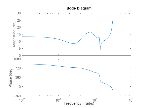
    Plot the Bode response.

    bode(sys)

    Create the specification object.

    R = reducespec(sys,"balanced");

    Notice that reducespec does not perform any computation and creates only the object. This allows you to set additional options before running the model order reduction algorithm, such as relative error control as the algorithm objective.

    R.Options.Goal = "relative";

    For balanced truncation, you can visualize the contributions in terms of the Hankel singular values or normalized energies. By default, the view function plots Hankel singular values.

    view(R)

    For this example, select an order of 15 since it is the first order with a relative error less than 1e-4. In general, you select the order based on the desired absolute or relative fidelity. Then, compute the reduced-order model.

    rsys = getrom(R,Order=15);

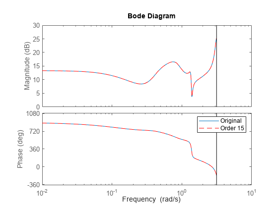
    Plot the Bode response of both models.

    bode(sys,rsys,'r--')
    legend("Original","Order 15")

    This example shows how to customize the state contribution plots obtained using the view function in the model order reduction workflow.

    For this example, create a model order reduction specification for a dense LTI model using the balanced truncation method. Generate a random discrete-time state-space model with 40 states.

    rng(0)
    sys = drss(40);

    Create a specification object and compute the information.

    R = reducespec(sys,"balanced");
    R = process(R);

    Visualize the Hankel singular values.

    view(R)

    To customize the plots for balanced truncation methods, you can use hsvoptions properties as input arguments.

    h = view(R,"sigma",YScale="linear")
    h =
    
    	resppack.hsvplot
    

    You can further customize this plot using the setoptions command.

    setoptions(h,'Grid','off')

    Input Arguments

    collapse all

    Model order reduction specification object created using reducespec, specified as a BalancedTruncation or SparseBalancedTruncation object.

    Plot type, specified as one of these strings.

    • "sigma" — Bar chart of Hankel singular values and associated error bounds.

    • "energy" — Bar chart of normalized state energies.

    If you do not specify this argument, the functions uses "sigma" for balanced truncation objects.

    Output Arguments

    collapse all

    Plot handle object, returned as an hsvplot object.

    Use setoptions with this handle to customize the plot. For example, setoptions(h,'Grid','off'). For a list of available options, see hsvoptions.

    References

    [1] Benner, Peter, Jing-Rebecca Li, and Thilo Penzl. “Numerical Solution of Large-Scale Lyapunov Equations, Riccati Equations, and Linear-Quadratic Optimal Control Problems.” Numerical Linear Algebra with Applications 15, no. 9 (November 2008): 755–77. https://doi.org/10.1002/nla.622.

    [2] Benner, Peter, Martin Köhler, and Jens Saak. “Matrix Equations, Sparse Solvers: M-M.E.S.S.-2.0.1—Philosophy, Features, and Application for (Parametric) Model Order Reduction.” In Model Reduction of Complex Dynamical Systems, edited by Peter Benner, Tobias Breiten, Heike Faßbender, Michael Hinze, Tatjana Stykel, and Ralf Zimmermann, 171:369–92. Cham: Springer International Publishing, 2021. https://doi.org/10.1007/978-3-030-72983-7_18.

    [3] Varga, A. “Balancing Free Square-Root Algorithm for Computing Singular Perturbation Approximations.” In [1991] Proceedings of the 30th IEEE Conference on Decision and Control, 1062–65. Brighton, UK: IEEE, 1991. https://doi.org/10.1109/CDC.1991.261486.

    [4] Green, M. “A Relative Error Bound for Balanced Stochastic Truncation.” IEEE Transactions on Automatic Control 33, no. 10 (October 1988): 961–65. https://doi.org/10.1109/9.7255.

    Version History

    Introduced in R2023b