How to Design and Simulate Motor Control Algorithms | Field-Weakening Control of PMSM with Simulink, Part 2
From the series: Field-Oriented Control of PMSMs with Simulink
In the second video of the series on Field-Weakening Control (FWC) for permanent magnet synchronous motors (PMSMs), we focus on designing and simulating control algorithm for PMSM. We will see how to use Motor Control Blockset™ reference examples as a starting point for implementing FWC algorithm for PMSMs. We will learn how to use desktop simulation to test and verify the algorithm. You can then reuse the same models to generate and deploy embedded code.
Published: 14 Apr 2021
Now, let's starting to view orientation control algorithms for brushless motor. As you can see from this overview system that [INAUDIBLE] diagram, we differentiate the control algorithm and physical system by collars. From the control side, there are many components, such as Park, Clark Transformation to cover current and voltage between stationary reference front and synchronize reference front. On the outer loop, we have speed controller, in the loop, current controller. To do close with control, we also have position or speed as a feedback for either sensor decoding logic or box observer, for those of you who are interested in senseless control.
To make the presentation more interesting, now, instead of showing you the implementation of fuel or inflation control, I would like to show you how do we design Maximum Torque Per Ampere, MTPA, with the weakening control. So now, the output of speed control and the input of the current controller is embedded with MTPA and fuel weakening. In this case, the current reference of q and b gases are calculated based on MTPA and fuel weakening algorithms to achieve maximum torque and minimal losses.
So let's quickly refresh back. What's Field-Weakening Control on brushless motors? What does it mean, and what's the motivation of doing that? Typically, in FOC we run the motor within a limit off base b. Before some application, we'd like to run motor beyond on the base speed, where the back emf will increase and is more than supply voltage. So the idea of Field-Weakening Control is to help us achieve higher speed without hitting lower voltage.
So we manipulate the axis theta current to be a negative value, which means we reduce the fuel current so that apply stator magnetic field is in the opposite direction to the rotor magnetic field. Turns out, the resulting magnetic field is reduced. Now, the back emf is reduced. So those reduced rotor flux linkage, which allows the motor to run at both the base b.
In order to achieve maximum torque per ampere, MTPA, is to increase the efficiency of the machine and to minimize the state of recurrent losses, as shown here on the right side of the figure. The blue concave curve shows the concentric line, indicating all IQ and IB pair force along those lines produce the same amount of total, but only concentric line intersect with the MPPL lines and the other operating points that can achieve MTPA.
So now, we have an accurate plan model and are ready to design all the controller. We will start with putting together a free orientation control algorithms with MTPA and be a weakening capability, including sensor decoder or observers if you want to implement census control.
So let's take a look through our model. Here, we have our speed controller that compute IQ and IB reference to track desire speed. One seemed to notice that the field weakening and MTPA control reference has been implement here. The torque and speed reference are input variables. The output IQ
and IB are calculate based on MTPA trajectory to produce desired optimum torque with minimum current magnitude.
Also, as we look closer, we can enable or disable the vehicle weakening control, depends on the operating speed condition. Now, we are never too close to the fuel orientation current control system. We have [INAUDIBLE] based vector generator. And that's as we dive into the IQ and IB PI regulator, we can see a Field-Weakening control is implement to control the IB reference. Remember, we have to inject a negative current to reduce the back emf voltage.
Next, I will navigate to a [INAUDIBLE] system that is sensor processing for current and position measurement. In the position measurement, you can see how we decode quadrature encoder readings using blocks from Motor Control Blockset. And here, I'm showing you how we computed UP cycles are written to PWM drivers on the microcontroller. Here, I'm also showing you the inverter and motor play model, so we can round close loops in relation.
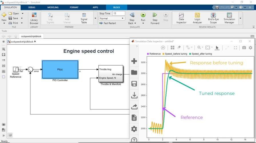
Now, I would like to show you a workflow how to tune the loop gains for current and speed controller. One thing to notice is that all shipping demos from Motor Control Blockset, including the one here, come with the scripts that run automatically when the motor initialize before simulation or cogeneration. As shown in the script, here, we are setting up our sample rate, loading the estimate motor parameters in computed offset for the sensors.
So after the perimeter has been set up, we can use the provided utility that will ultimately compute over load gains based on motor and inverter parameter values. A script used computer gains and motor parameter values to automatically compute gains and phase margin for our [INAUDIBLE] body clock instead, responds, by using the control system tool box. And in the workspace, here, you can see we have our estimate motor parameters, sensor offset, and computed bookings.
So for the tuning the loop gains, Motor Control Blockset not only have empirical calculation, but also, FOC Autotuner can ultimately compute or gain space on the bandwidth and base margin you specify. You can also use other tools for Simulink Control Design to control games. So let's move them round our control algorithm in closed loop simulation.
As you can see from the top left corner, we can simulate the plan model with switching event by choosing Simscape Electrical, then, comparing with the simulation without using every value inversion model. Once the simulation is over, we can look at the data inspector.
So we are going to look at the speed response, IQ response, phase a voltage and current, and, finally, post width modulation waveform. As you can see on the speed command tracking, on first one it looks pretty good with the speed feedback followed as we come in. And let's look at the second row of the [INAUDIBLE] command tracking response. We can see those switching effect, where highlighted in yellow, and the blue line shows the current model by average value inverter.
Why are we tuning? We can clearly see the [INAUDIBLE] switching in the phase voltage and current plot. And finally, when we will get a PWM modulation waveform, there's not a big significant difference between those two rounds, but the bottom line is that we can bring a different level of stability depends on our testing area. As we do leave here, we can clearly see the effect of switching events.


