Supervisory logic design | Drilling Systems Modeling & Automation, Part 5
From the series: Drilling Systems Modeling & Automation
Drilling systems of today are designed around the human operator; the human verifies that equipment is reacting per applied set-points and interprets sensor readouts to decide proper actions. For future drilling control systems, it is likely that the greatest drilling cost savings will come from applications that not only use control to automate the drilling machines and equipment, but also to automate decisions in the supervisory control of these machines and equipment. The equipment controls are preprogrammed to act repeatedly based on defined inputs and known states, such as the auto driller.
In this video, we design an auto driller that senses the mass & current position of the top drive and automatically adjusts the motor speed setpoint. This is done by implementing the look-up table as a supervisory controller using state-based logic. We show how the supervisory control algorithm steps through the drawworks operating states such as raising and lowering the drillstring and stopping. This is implemented in Stateflow.
Stateflow enables you to design and develop supervisory control by building state charts. You can visualize system behavior using state diagram animations to highlight active states and transitions in your charts. Stateflow also allows you to graphically describe how MATLAB® algorithms and Simulink® models react to input signals, and time-based conditions.
Published: 2 Jul 2020
Hi, and welcome back. My name is Jonathan LeSage, and I'm an application engineer with The MathWorks. Today, we're going to discuss how we can start to implement state-based logic in Simulink for our digital twins for testing control logic.
For the example that we've been using in this video series, we've been putting together a drawworks drilling system. And we've been focused on the auto driller limits, so how fast we can raise and lower this drilling system without us actually crowning out up top or bottoming out on the bottom given how much weight we have.
In the last video, we saw how we could use our digital twin to actually sweep wide parameter spaces, operational spaces, and then come up with limits on what our actual maximum speed commands can be. Today, we're going to look at how we can start to implement this logic in a state-based chart.
All right. So let's take a hop over to Simulink. So here's where we left off. This is our drawworks system. I'm going to go ahead and run the simulation again so we can get a sense of what's going on. Our system's going to lift the hoist up without crowning out. We're not going to actually impact the top. We're going to go up as fast as we can. And again, we're going to lower as fast as we can without bottoming out.
Recall that our drive here actually has torque-speed curve limits. And so, depending on the speed and the torque requirements-- and that's, of course, dictated by how heavy this load is-- we're going to have to operate this in different ways.
Now, the operational logic, the safety-critical aspect of this is implemented in this state chart. So we have this auto driller mode that's basically raising the hoist. Once we get to the top, we have this add pipe and make section. Then we have a lower and drill, and then we have a break string.
You'll notice that, in the raise and the lower states, we have this energy speed limiter, which basically takes in a speed command-- in the lower case, minus 1,500 RPM, or in the top case, 1,500 RPM-- and the current mass and the current position, and it will dictate what the actual limit can be. And this is coming from that lookup table that we built last time.
Now, this chart that we're executing here, as the drawworks raises and lowers, you can see the state that we're in. And this is a tool called Stateflow. Now, Stateflow lets us build these state-based flow charts quickly and easily in Simulink. And you'll notice, at the top level, they appear just as a Simulink subsystem.
So I can have numeric inputs, Boolean inputs, and these can provide outputs to different physical systems like drives or other components, just like you would have, say, a PLC or something in the field receive measurements from your equipment and then decide and do actions and provide outputs. OK? Now, we're going to take a look at how to build this chart in a little more detail.
All right. Let's see how we can create one of these charts from scratch. So we're going to go over to Simulink here. Now, we're going to start with a blank model. But if you knew you were just going to be focusing on a state machine, you could scroll down here to the Stateflow starter templates and get a little simple Stateflow chart started or even a hierarchical chart. But we're going to go ahead and use a blank model, build it from scratch.
Now, if we open up Simulink and go into the library browser, we can find the state diagrams under the Stateflow library. You'll see there's a few different types. We're going to be focused primarily today on the chart. Chart gives you the most flexibility. The other styles of modeling are a little more for restrictive styles of modeling for very efficient kind of truth table-type things.
Now, once you've double clicked on it, this is kind of like a subsystem in Simulink. Now we're inside of this subsystem, and we can start to place components. Now, we can place things like states, so we could call this off. We can copy and paste that over here. That creates an on state. And it's kind of nice that those things update for us.
We could say maybe this is on, and then we could expand this out and then have some substates inside of this. So this could be raise hoist. Then we could have lower hoist, for example. Maybe we can have an intermediate state, something like at top. And maybe one more, at bottom, just to kind of serve as an example.
All right. And I'm just going to spread these out a little bit just to make things a little more interesting. And so these are the different states we have in our machine. So we have an off state, we have an on state. And within on, we have some substates, raising, lowering, we're at the top, we're at the bottom.
The other aspect of a state machine is the connections or junctions, and these are basically the logic that must be true to transition from one state to the other. So we can have a condition. Maybe we can have a thing called on switch equals 1. So if our on switch is 1, we go into the on state.
And then, once we're in the on state, we raise the hoist. And then we can basically raise hoist until x is greater than 10. And then, if we're greater than 10, we're at the top. And once we're at the top, maybe after a certain amount of time, we can transition to lower. So we can say, maybe after five seconds-- so you can have temporal conditions as well-- lower the hoist.
And then we can go to bottom, so x is maybe less than 0, we're at the bottom. And then, finally, we can go from bottom back to top. And we can say that occurs after five seconds as well. And I need to make sure I don't do typos. OK.
All right. Now, if I go ahead and try to run this chart, we're going to see we get an error message. And this error message, which is showing up off my screen, actually says that our chart has unresolved symbols. And actually, Simulink, in this case, is giving me a little helper saying that it's found unresolved symbols, but it thinks it knows what I'm trying to do with these. It says I'm using the on switch as an input, and same with x. And in this case, I agree, so I'll say OK.
And now, after doing that, we'll notice that my chart block has two input ports, one for on switch and one for x. And so I could add a constant block here maybe for my on switch, just leave it as a 1. And then maybe, for x, we can do something like a sinusoid just to keep things interesting. And we will make it 5, and it will go up and down 5.1. So it'll go up and down below 0, and that should be good.
And if we push play, now we should see our chart actually start to execute things. And we saw it executed quite quickly, and that's typically OK. If you want to slow this chart down, you can actually go into the animation here under the debug mode and slow this down so you can more easily see the transitions, so raise hoist, at top, after five seconds, lower hoist, and then we actually ran out of time in this case.
Now, those are for inputs. We could also add additional things inside these states. So raise hoist, maybe we want to have some code executed when we are raising the hoist. And so maybe we want to have something like our speed command. We could say that equals 1,500 like we did in the other one. And then maybe lower hoist equals minus 1,500.
And so this is just kind of your standard MATLAB syntax. And at top, maybe do a command equals 0. Same thing, w command equals 0 at the bottom as well. And over here in off, we can give the same thing, w command equals 0. Clearly, we don't want it to be moving when we're off.
Again, I'll try to run it. We'll see the unresolved states. It says, w command, looks like we're using that as an output. And that's correct, we are. And so now, if we go back, we'll see that w command here is an output that we could feed into something like a scope. And we can connect that up, and we can push play. And now we'll see what our w command is during the entire simulation. It's 1,500, 0, and then minus 1,500. It gives us an idea of what's actually going on with the simulation.
All right. For the last piece of this, we talked about the energy speed limiter. And rather than build that from scratch, I just wanted to hop back to the completed chart. Now, there's a few ways that you can implement additional logic in your charts, especially if you have things like more complex numeric calculations.
So things like lookup tables where maybe you want to use the Simulink blocks, you can have what's called a Simulink function directly in your chart. This is going to act just like a Simulink block, but it will be kind of a function that you call from your Stateflow charts here. So you'll see energy speed limiter here. It has three inputs, so it just corresponds to the three inputs here, and two outputs, which correspond to the two outputs here.
Now, you could do this graphically with these Simulink functions, but you also have the option to use something more like a MATLAB function where, once you double click here, it will take you into the MATLAB environment and you can script things out more programmatically if that's more your style.
Now, you'll notice that, once we're in here, the inputs map to the input ports here-- w command, m, and x-- and the outputs here map to the output ports. So every time that our Stateflow chart enters this state and requests this function here, the current numerics here get passed into this function, get fed through this Simulink function block, and then pass out as outputs here, which then get passed back into our Stateflow chart.
The beauty with all of this is, of course, we can do verification and validation on this. We can check to ensure that we're not having any divide by zero issues. And we can also check and then also, finally, generate code from the Stateflow diagram to be used on our actual hardware.
And so this could be processors that use embedded C or other processors like PLCs that use a language like structured text. So once we've tested and validated this state chart here with our digital twin simulation, we can actually leverage that in the field with our actual hardware. And that's what we're going to see next.


